Allele Specific Copy Number Inference • signals

library(signals)

Background

This vignette illustrates how to perform allele specific copy number inference with DLP+ data. However the method should be generally applicable to any single cell copy number method. The input requirements are discussed below.

Data

The data needed to perform the allele specific copy number inference are binned copy number data and cell specific haplotype calls. The copy number data and the haplotype data should use the same bins.

A small test data set of 250 cells is provided with the package, we’ll load this data and inspect these 2 dataframe.

data(haplotypes)
data(CNbins)

head(CNbins)
#>   chr   start     end reads     copy state               cell_id
#> 1   1 2000001 2500000   536 2.960868     2 SA921-A90554A-R03-C44
#> 2   1 3000001 3500000   499 2.603584     2 SA921-A90554A-R03-C44
#> 3   1 4000001 4500000   569 2.216388     2 SA921-A90554A-R03-C44
#> 4   1 4500001 5000000   524 2.039672     2 SA921-A90554A-R03-C44
#> 5   1 5000001 5500000   576 2.210792     2 SA921-A90554A-R03-C44
#> 6   1 5500001 6000000   516 2.028686     2 SA921-A90554A-R03-C44

The haplotype data comes in long format, but the package requires data in wide format so we will use the helper function format_haplotypes_dlp to convert the data to the correct format, this function will also remove any bins present in the haplotypes data frame that is not present in the CNbins data frame.

haplotypes <- format_haplotypes_dlp(haplotypes, CNbins)
head(haplotypes)
#>                  cell_id chr   start     end hap_label allele1 allele0
#> 1 SA1090-A96213A-R20-C13   1 2000001 2500000       101       0       3
#> 2 SA1090-A96213A-R20-C13   1 2000001 2500000       104       0       1
#> 3 SA1090-A96213A-R20-C13   1 2000001 2500000       106       0       3
#> 4 SA1090-A96213A-R20-C13   1 2000001 2500000       108       0       4
#> 5 SA1090-A96213A-R20-C13   1 2000001 2500000       112       0      15
#> 6 SA1090-A96213A-R20-C13   1 2000001 2500000       113       0       1
#>   totalcounts
#> 1           3
#> 2           1
#> 3           3
#> 4           4
#> 5          15
#> 6           1

Inference

The output of signals is allele specific states per bin. signals has 2 options to perform this inference, the first, callAlleleSpecificCN, infers allele specific states using mirrored B allele frequencies as is typically done in bulk whole genome sequencing. This infers states of the form A|B where B < A. The second option, callHaplotypeSpecificCN takes into account the possibility that different alleles may be lost or gained in different cells. In order to identify these events, signals clusters cells and infers the haplotype phase based on regions within clusters that have large allelic imbalance. The output for this method therefore allows for B>A. We would generally recommend using callHaplotypeSpecificCN as this is more informative, so this vignette largely focuses on this option. callAlleleSpecificCN works in a similar way.

`callHaplotypeSpecificCN`

hscn <- callHaplotypeSpecificCN(CNbins, haplotypes)
#> VGLM    linear loop  1 :  loglikelihood = -312941.0231
#> VGLM    linear loop  2 :  loglikelihood = -308976.287
#> VGLM    linear loop  3 :  loglikelihood = -308423.1945
#> VGLM    linear loop  4 :  loglikelihood = -308397.0858
#> VGLM    linear loop  5 :  loglikelihood = -308396.6937
#> VGLM    linear loop  6 :  loglikelihood = -308396.6901
#> VGLM    linear loop  7 :  loglikelihood = -308396.69

As a sanity check we can plot the B allele frequency (BAF) as a function of inferred state. We would expect to see a distribution around the expected value which is exactly what we see below.

plotBAFperstate(hscn, maxstate = 10)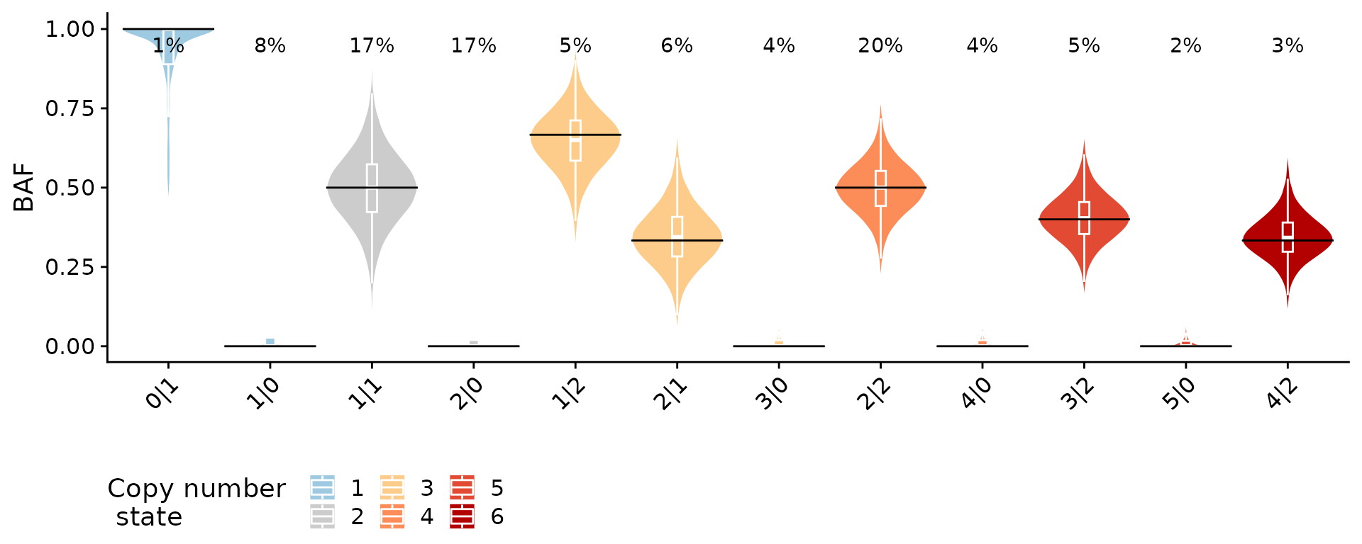

Now we can plot the copy number heatmaps. First we’ll plot the heatmap based on copy number states. We can provide the plotHeatmap function with a tree in newick format to plot an ordered heatmap and/or a dataframe with cluster assignments. By default the plotHeatmap function does some clustering using hdbscan if neither of these is provided.

cl <- umap_clustering(hscn$data)

plotHeatmap(hscn, 
            plotcol = "state", 
            clusters = cl$clustering,
            tree = cl$tree, 
            reorderclusters = TRUE, #order according to tree
            plottree = FALSE) #do not plot the tree but keep the ordering )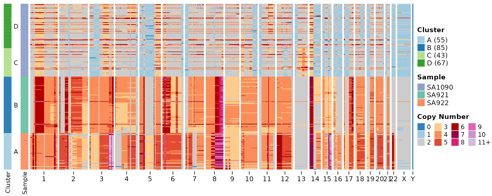

Now we can plot some heatmaps to visualize the allele specific state. This heatmap plots the B allele copy number state.

plotHeatmap(hscn, plotcol = "B",
            clusters = cl$clustering,
            tree = cl$tree, 
            reorderclusters = TRUE, #order according to tree
            plottree = FALSE) #do not plot the tree but keep the ordering )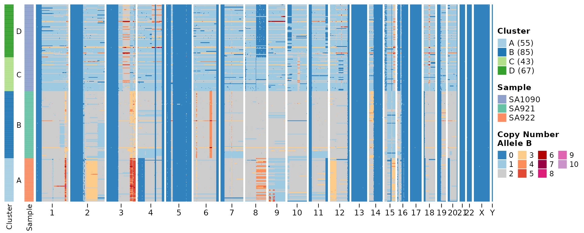

Discrete representation of allelic imbalance:

plotHeatmap(hscn, 
            plotcol = "state_phase", 
            clusters = cl$clustering,
            tree = cl$tree, 
            reorderclusters = TRUE, #order according to tree
            plottree = FALSE) #do not plot the tree but keep the ordering )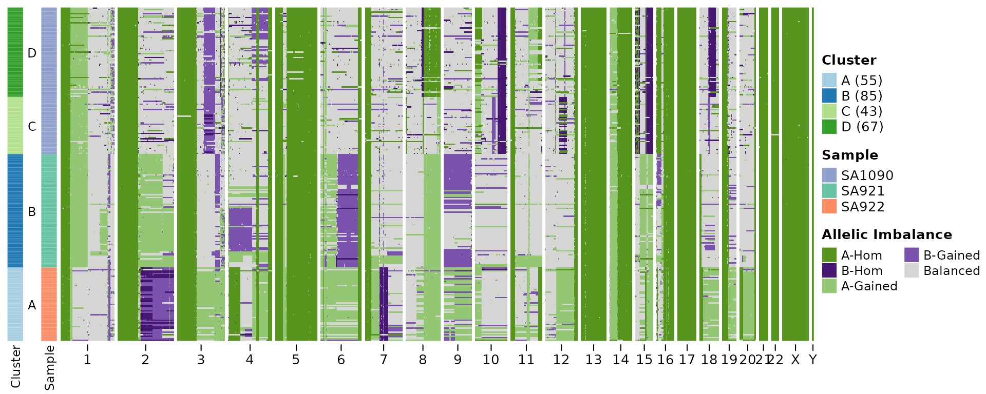

There are also some function to plot per cell BAF and state plots. You can specify a cell, or the default will take the first cell in the data frame.

plotCNprofileBAF(hscn, cellid = "SA921-A90554A-R03-C44")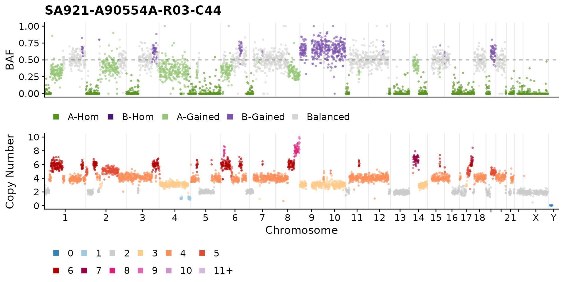

Here we’ll plot an equivalent plot merging data across cell clusters using the utility function consensyscopynumber. Here, the cell_id column becomes the


consensus_clusters <- consensuscopynumber(hscn$data, cl = cl$clustering)

plotCNprofileBAF(consensus_clusters, cellid = "A")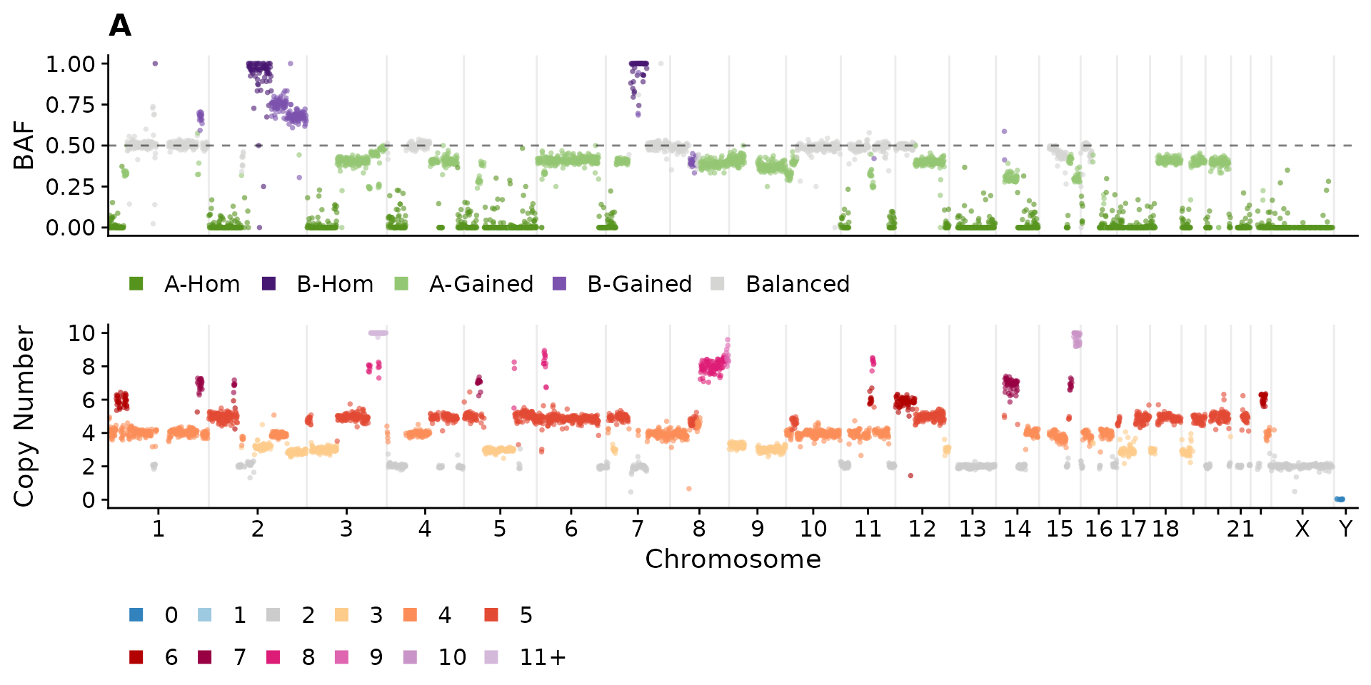

The object returned by the inference function is of type hscn, if you want to pull out the data to use in your own scripts you can just do hscn$data. This will return a data.frame similar to the input data frames but with additional columns specifying the allele specific states.