Basic scDNAseq analysis • signals

library(signals)

Background

Although this package was put together to infer allele or haplotype specific copy number in scDNAseq data, it has a lot of methods for visualization and analysis that should be useful for any type of scDNAseq data, including when you only have total copy number calls. Here we’ll go through the available plotting functions and various utilities to summarize the data.

Data input

The main requirement is a dataframe with the following columns: chr, start, end, cell_id, state, copy. state is the inferred total copy number state. copy values are GC-correceted, ploidy corrected normalized read counts that would be used to infer the states. This may difer depending on the tool you use. We provide some example data (CNbins) with this package. Most functions will work with either this kind of dataframe or a signals object, here we’ll just use the CNbins dataframe.

Plotting

Single cell profiles

The first thing we can do is plot single cell copy number profiles.

plotCNprofile(CNbins, cellid = "SA921-A90554A-R03-C44")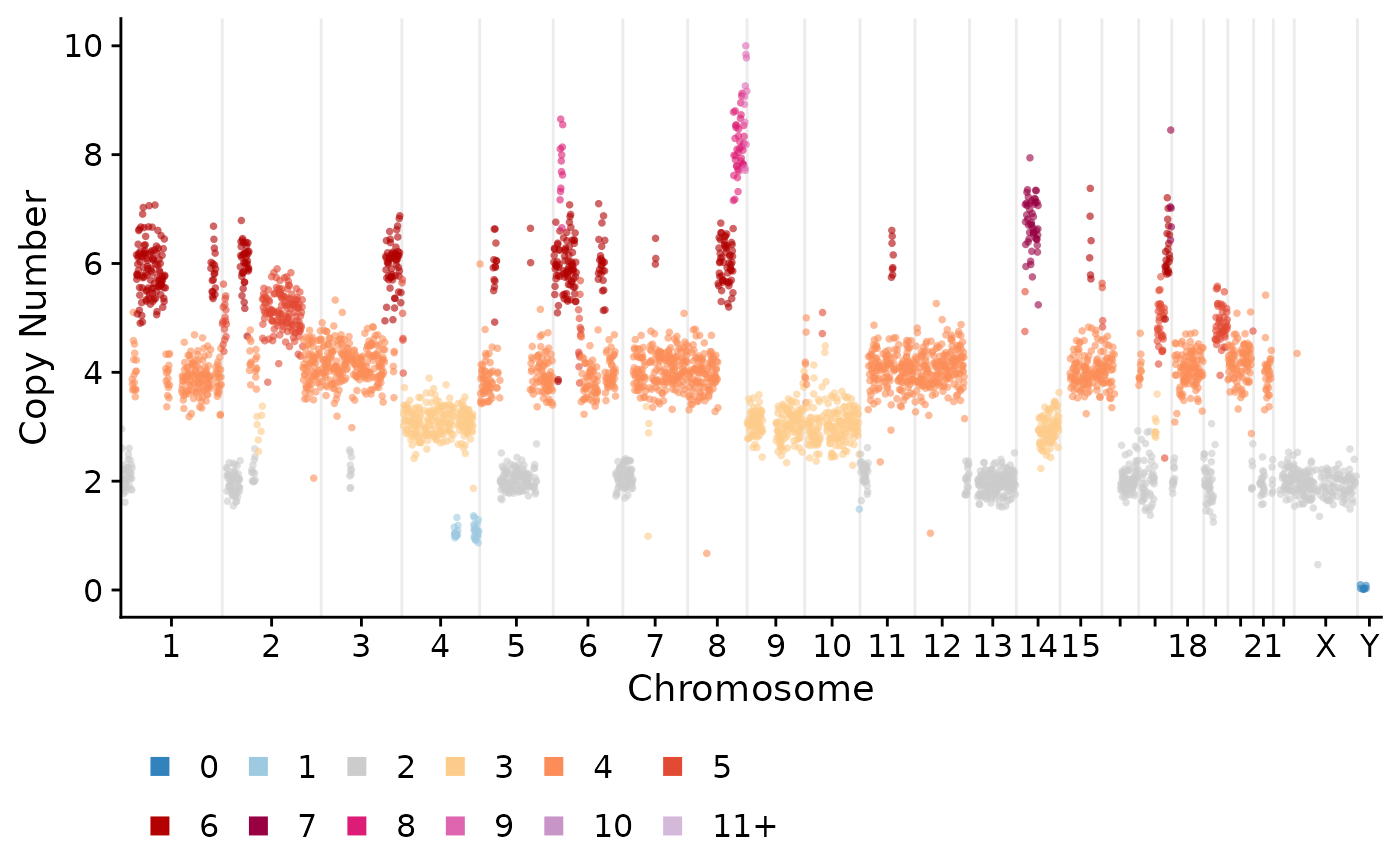

These can tweaked in various ways, including modifying the y-axis, only plotting certain chromosomes or changing the point size etc:

plotCNprofile(CNbins, cellid = "SA921-A90554A-R03-C44", y_axis_trans = "squashy", maxCN = 25, chrfilt = c("6", "7", "8"), pointsize = 2)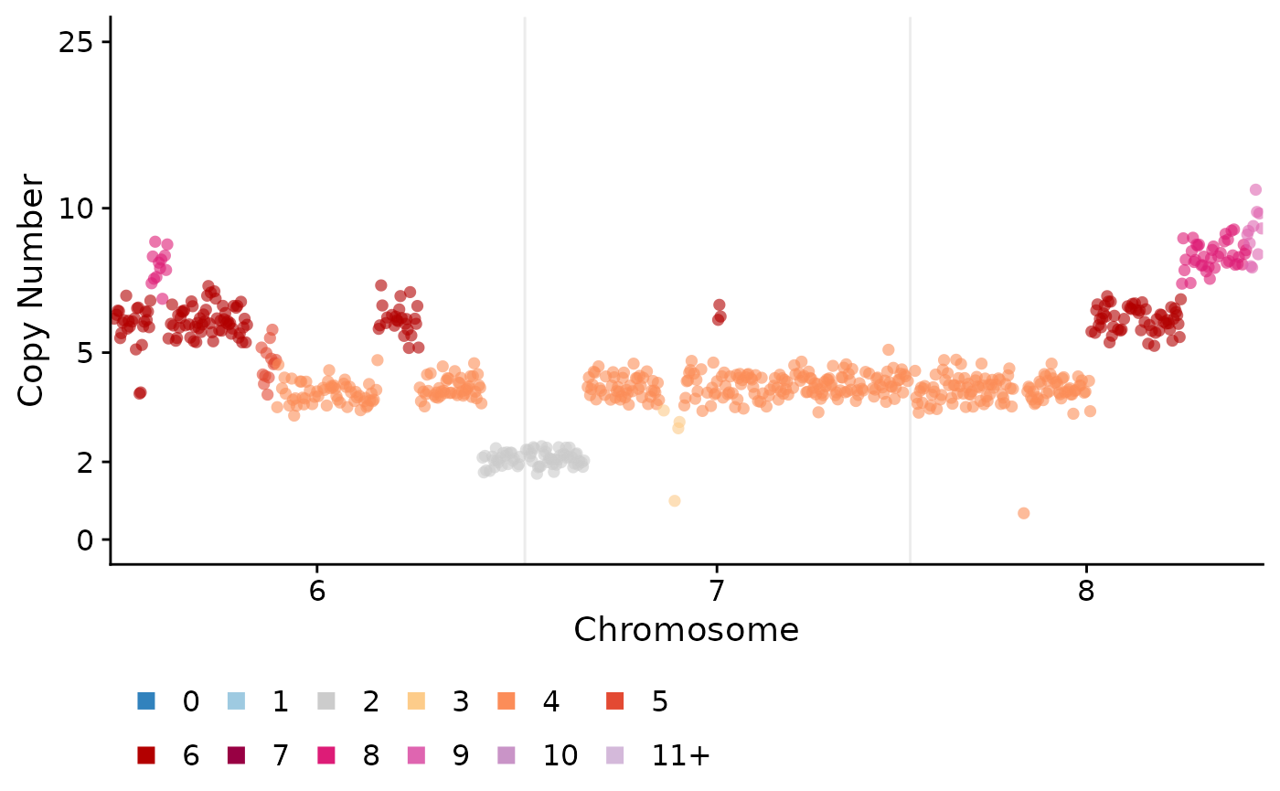

We can also plot all the cells using the plotHeatmap function. This can optionally take in a phylogenetic/clustering tree in newick format. If you don’t have this you can use the umap_clustering function to cluster your data using umap and hdbscan.

clustering <- umap_clustering(CNbins, field = "copy")

Heatmaps

Then we can use this output in the plotHeatmap function. If you leave the tree and clustering options empty then plotHeatmap will fall back to use umap_clustering.

plotHeatmap(CNbins, tree = clustering$tree, clusters = clustering$clustering)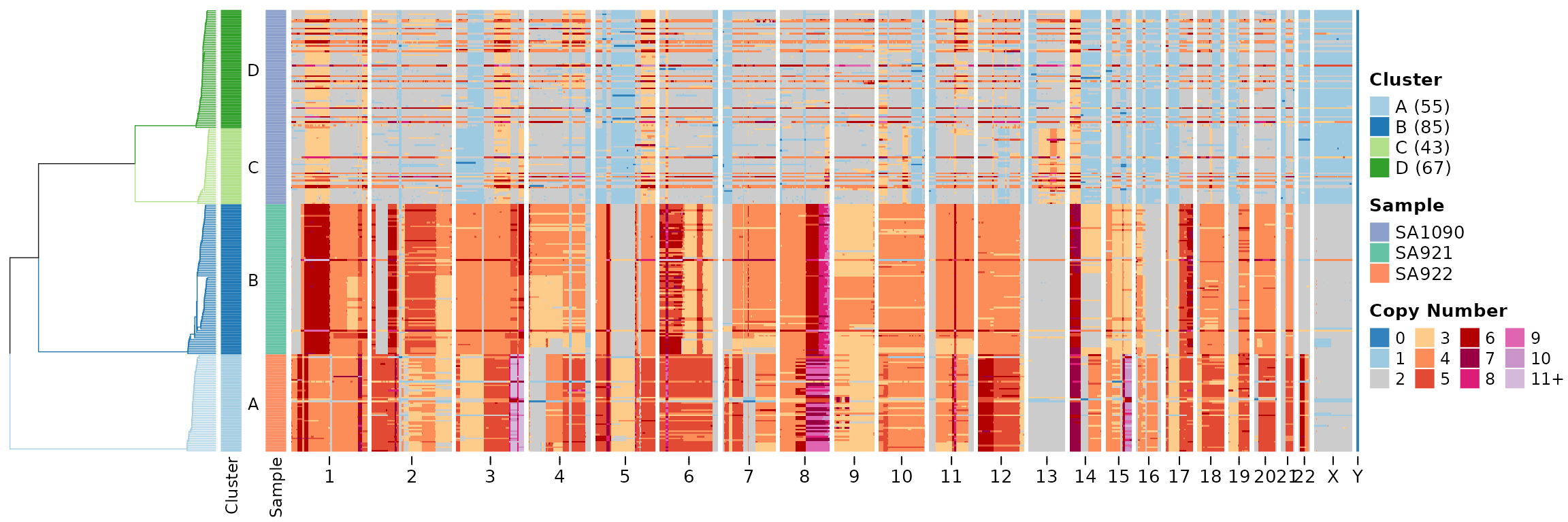

The default is to plot the state column, we can change this to plot the copy raw data column.

plotHeatmap(CNbins, tree = clustering$tree, clusters = clustering$clustering, show_clone_label = F, plotcol = "copy")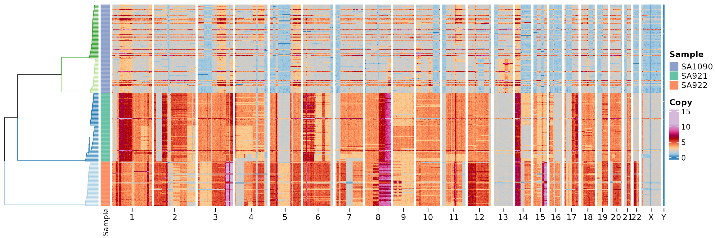

Alternative clustering with Leiden

An alternative to UMAP+HDBSCAN clustering is the Leiden algorithm, which uses PCA + k-nearest neighbor graphs for community detection. This approach can produce different clustering results and offers more control over the tree structure.

leiden_clustering_result <- leiden_clustering(CNbins, field = "copy", k = 15, resolution = 0.7, seed = 42)

We can visualize the Leiden clustering results in a heatmap. By default, leiden_clustering uses tree_type = "centroid", which creates a tree where cells within each cluster form a flat star structure (all cells at the same depth within their cluster):

plotHeatmap(CNbins, tree = leiden_clustering_result$tree, clusters = leiden_clustering_result$clustering)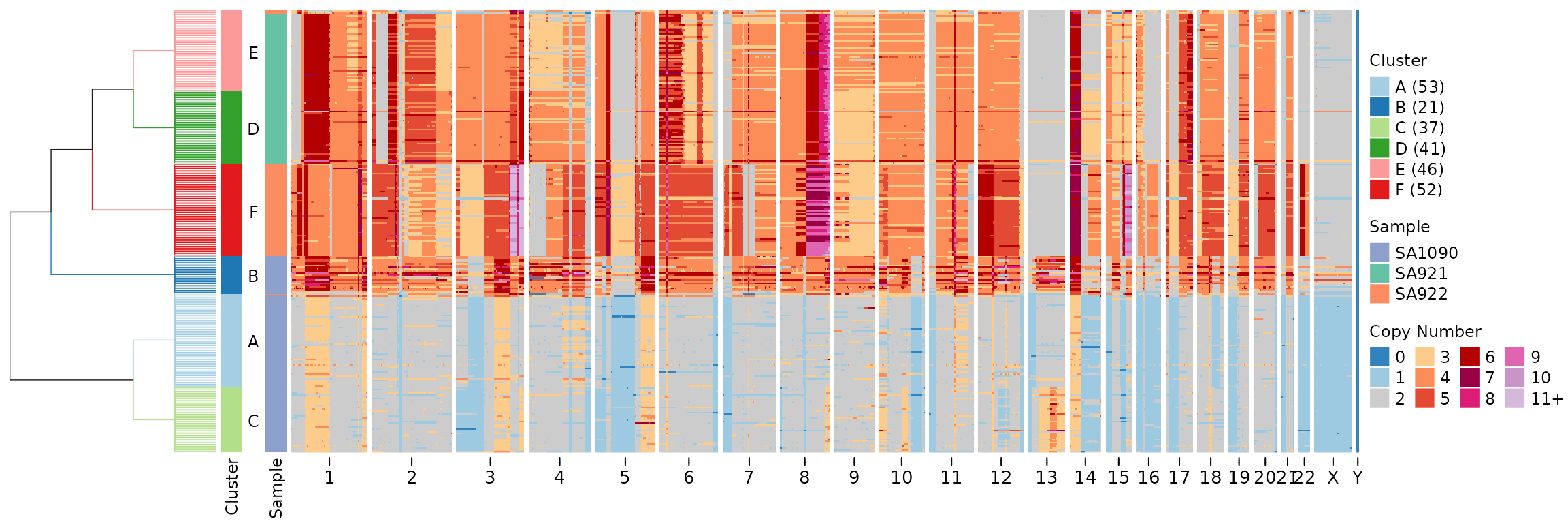

For a more detailed cell-level tree that adds hierarchical structure within clusters, we can use tree_type = "cell". This creates subtrees via hierarchical clustering within each cluster and grafts them onto the backbone tree of cluster centroids:

leiden_cell_tree <- leiden_clustering(CNbins, field = "copy", k = 15, resolution = 0.7, tree_type = "cell", seed = 42)

plotHeatmap(CNbins, tree = leiden_cell_tree$tree, clusters = leiden_cell_tree$clustering)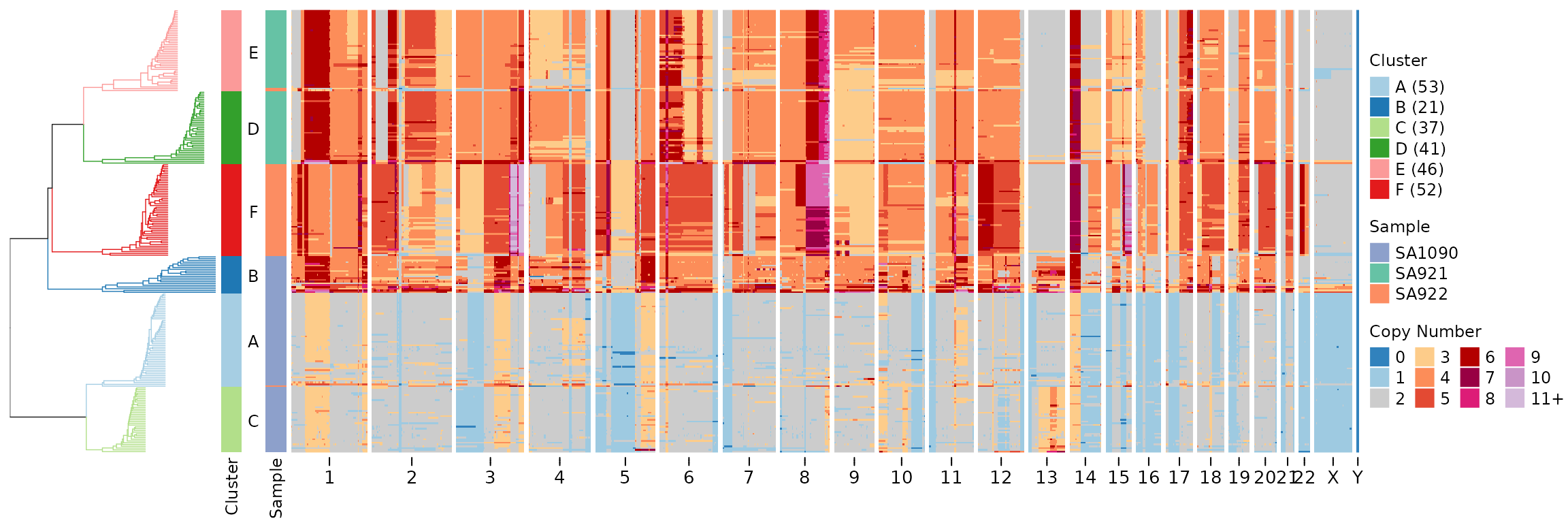

Both tree types preserve cluster blocks (cells from the same cluster are always adjacent in the tree).

Utilities

Compute consensus copy number profiles.

CNbins_consensus <- consensuscopynumber(CNbins, cl = clustering$clustering) #cell_id becomes clone_id

plotCNprofile(CNbins_consensus)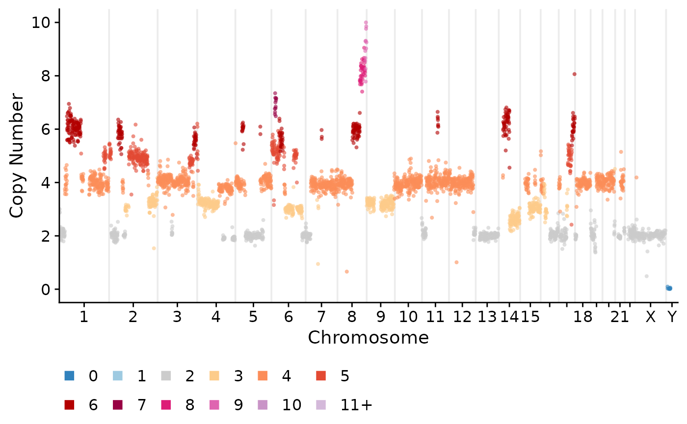

Create segmentation from binned data.

segments <- create_segments(CNbins)

Compute average copy number per chromosome or chromosome arm.

CNbins_chr <- per_chr_cn(CNbins)

CNbins_arm <- per_chrarm_cn(CNbins)