Beta-Binomial model for signals • signals

library(signals)

Background

This vignette demonstrates how to use a beta-binomial model instead of a binomial model for the HMM emission model.

Inference

data("haplotypes")
data("CNbins")
haplotypes <- format_haplotypes_dlp(haplotypes, CNbins)
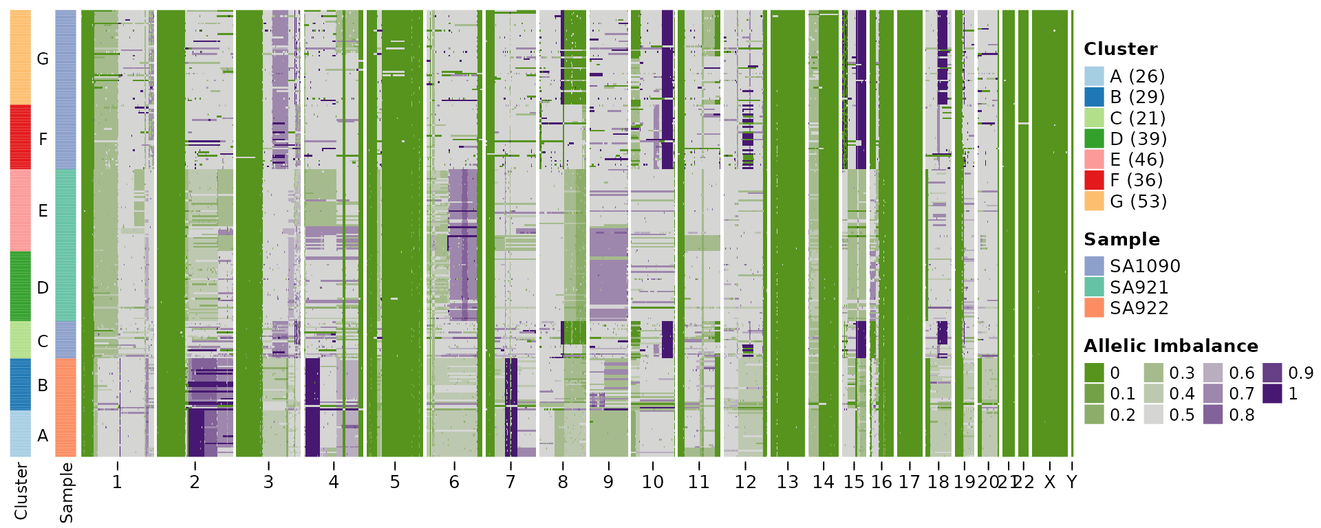
hscn <- callHaplotypeSpecificCN(CNbins, haplotypes, likelihood = "binomial")

print(hscn)
#> Haplotype specific copy number object 
#>  
#> Number of cells: 250
#> Bin size: 0.5 Mb 
#> Inferred LOH error rate: 0.018 
#> Emission model for HMM: binomial 
#> Average distance from median to expected BAF = 0.0025 
#> Average ploidy = 4 
#> Average number of segments = 79

hscn_bb <- callHaplotypeSpecificCN(CNbins, haplotypes, likelihood = "betabinomial")
#> VGLM    linear loop  1 :  loglikelihood = -312846.9331
#> VGLM    linear loop  2 :  loglikelihood = -308871.7299
#> VGLM    linear loop  3 :  loglikelihood = -308314.3828
#> VGLM    linear loop  4 :  loglikelihood = -308287.9087
#> VGLM    linear loop  5 :  loglikelihood = -308287.51
#> VGLM    linear loop  6 :  loglikelihood = -308287.5063
#> VGLM    linear loop  7 :  loglikelihood = -308287.5063

print(hscn_bb)
#> Haplotype specific copy number object 
#>  
#> Number of cells: 250
#> Bin size: 0.5 Mb 
#> Inferred LOH error rate: 0.018 
#> Emission model for HMM: betabinomial 
#>   Inferred over dispersion: 0.0096
#>   Tarones Z score: 179.167
#> Average distance from median to expected BAF = 0.0026 
#> Average ploidy = 4 
#> Average number of segments = 79

We see that the model inferred a modest degree of overdispersion in the data, but that this was siginificantly different from 0 dispersion (Tarones Z-score is high).

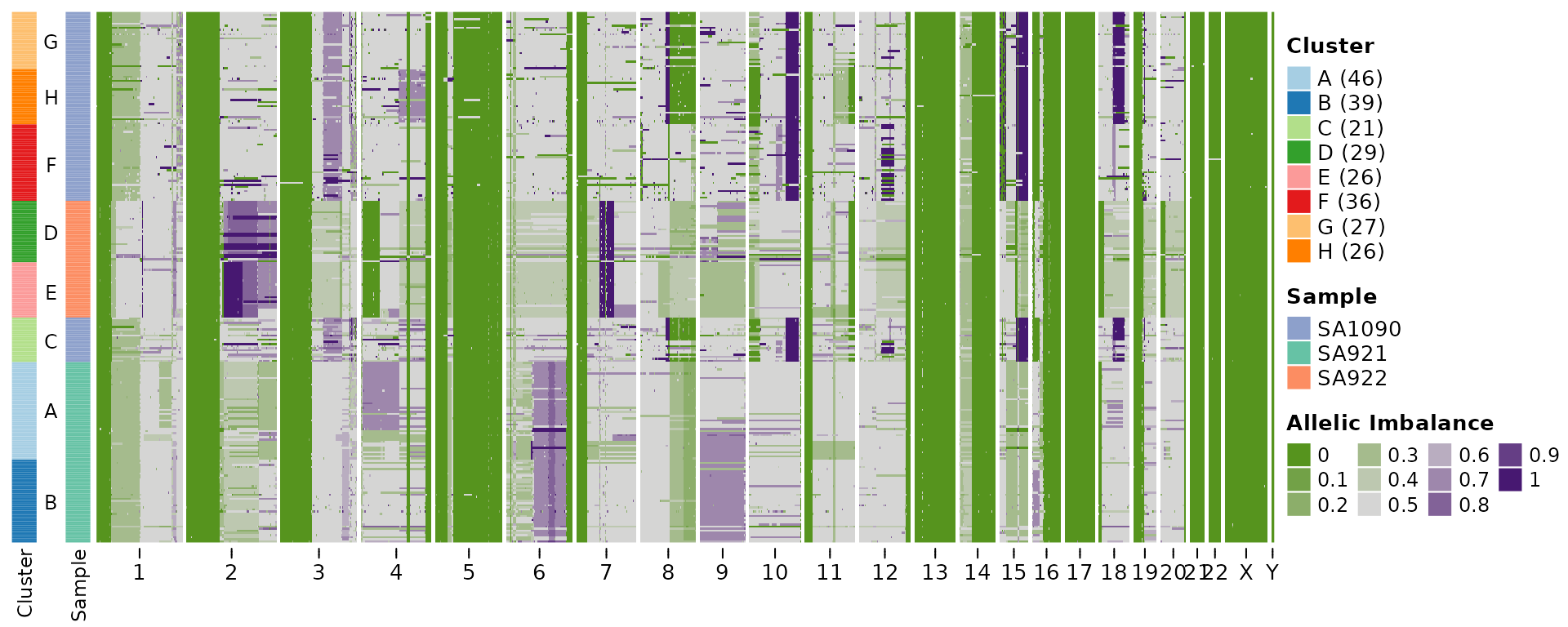
Below I’ll plot the heatmaps for the two output, which in this case are very similar.

Binomial model

plotHeatmap(hscn, plotcol = "state_BAF", plottree = FALSE, spacer_cols = 15)

Beta-Binomial model

plotHeatmap(hscn_bb, plotcol = "state_BAF", plottree = FALSE, spacer_cols = 15)

QC plot

To interrogate the difference between the binomial and beta-binomial models we can plot the BAF and overlay the two models.

plotBBfit(hscn_bb)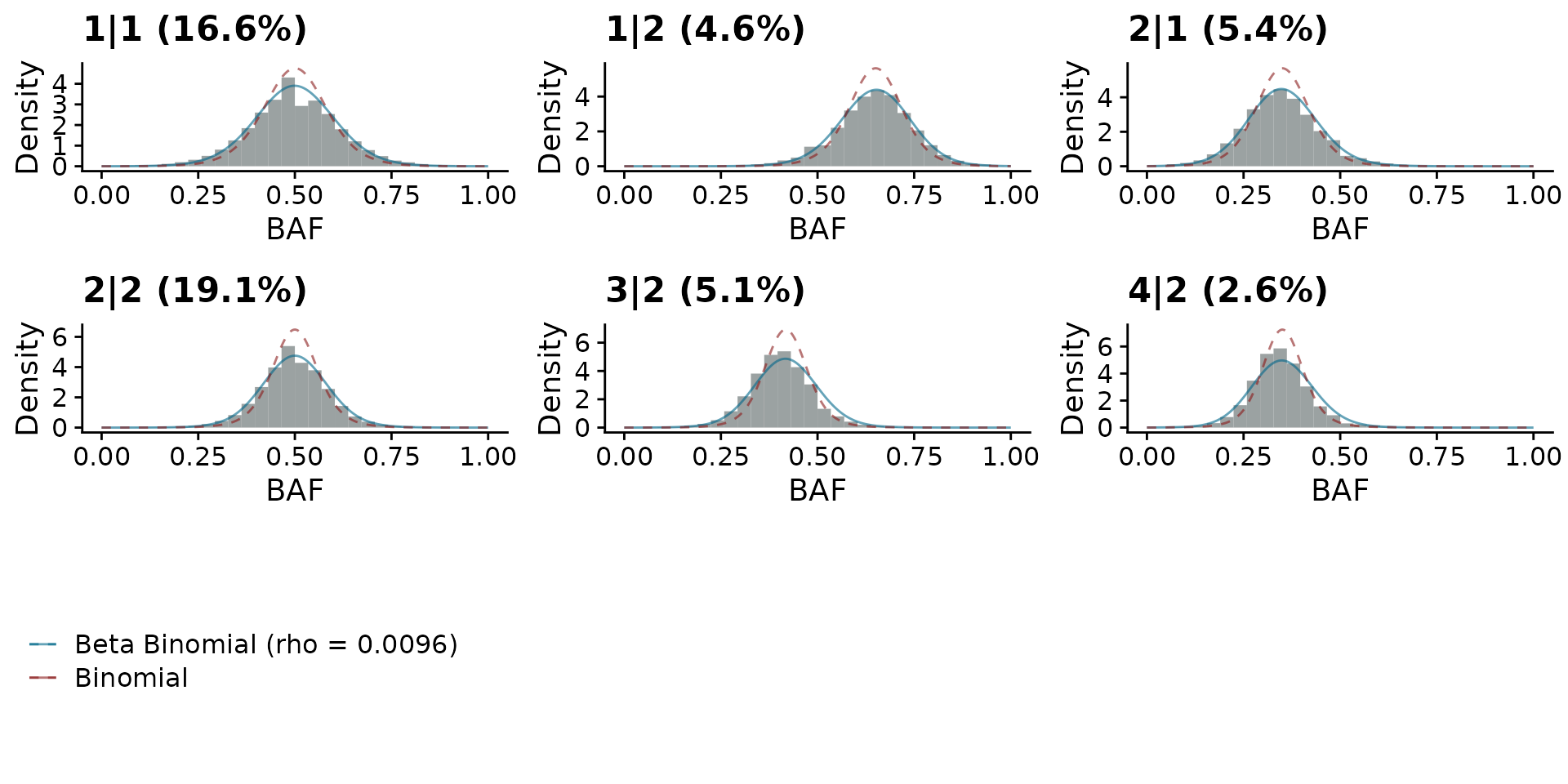

We can check how similar the results are by comparing the two dataframes. We find for this data that the results are very similar.

print(dim(hscn$data))
#> [1] 1093750      20
print(dim(hscn_bb$data))
#> [1] 1093750      20
all.equal(orderdf(hscn$data), orderdf(hscn_bb$data))
#>  [1] "Component \"alleleA\": 'is.NA' value mismatch: 17525 in current 17561 in target"    
#>  [2] "Component \"alleleB\": 'is.NA' value mismatch: 17525 in current 17561 in target"    
#>  [3] "Component \"totalcounts\": 'is.NA' value mismatch: 17525 in current 17561 in target"
#>  [4] "Component \"BAF\": 'is.NA' value mismatch: 17525 in current 17561 in target"        
#>  [5] "Component \"state_min\": Mean relative difference: 0.6273572"                       
#>  [6] "Component \"A\": Mean relative difference: 0.6281181"                               
#>  [7] "Component \"B\": Mean relative difference: 0.6525181"                               
#>  [8] "Component \"state_AS_phased\": 32952 string mismatches"                             
#>  [9] "Component \"state_AS\": 2977 string mismatches"                                     
#> [10] "Component \"LOH\": 1926 string mismatches"                                          
#> [11] "Component \"phase\": 29910 string mismatches"                                       
#> [12] "Component \"state_phase\": 30877 string mismatches"                                 
#> [13] "Component \"state_BAF\": Mean relative difference: 0.8574611"

Another thing we can check is the total number of segments identified by the HMM. Using the beta-binomial model should reduce the influence of any noisy regions and thus we might expect fewer segments. We do observe fewer segments in the beta-binomial model.

segs <- create_segments(hscn$data, field = "state_AS_phased")

segs_bb <- create_segments(hscn_bb$data, field = "state_AS_phased")

print(dim(segs))
#> [1] 38884     5
print(dim(segs_bb))
#> [1] 35477     5

Summary

With this dataset, the difference between the nbinomial model and beta-binomial model is minimal but produces a statistically superior fit, in lower quality datasets with for example lower depth of coverage the beta-binomial model may may provide more noticeable differences.