Structural variant visualization
SV_visualization.RmdplotCNprofile can draw structural variants on top of a
copy number profile. This vignette covers the data format it expects,
then works from a single SV up to whole-genome views with many.
The example data is the OV2295-derived cell line SA921:
CNbins holds the copy number, SVs holds
destruct breakpoint calls for the same sample.
data(CNbins)
data(SVs)

# CNbins bundles several samples; keep the one the SVs were called on
cn <- dplyr::filter(CNbins, grepl("^SA921", cell_id))
cell <- unique(cn$cell_id)[1]
SV data format
SV is a data frame with one row per breakpoint. Two
columns describe each breakend, plus the read support:
head(SVs, 3)
#>   chromosome_1 position_1 strand_1 chromosome_2 position_2 strand_2
#> 1            1   15699950        +            1   15581820        -
#> 2            1   16928143        -            1  120401537        -
#> 3            1   16969869        +            3   49728337        -
#>            type rearrangement_type read_count
#> 1   duplication        duplication          8
#> 2     inversion         unbalanced          9
#> 3 translocation unbalanced 6| Column | Required | Notes |
|---|---|---|
chromosome_1, position_1,
strand_1
|
yes | first breakend |
chromosome_2, position_2,
strand_2
|
yes | second breakend |
read_count |
for "lines_and_arcs"
|
supporting reads |
type, rearrangement_type
|
optional | used by the "curves" style |
Strands must be the characters "+" and "-".
Callers that store them as logicals need converting first, otherwise the
arcs are silently dropped:
SVs <- dplyr::mutate(SVs,
                     strand_1 = ifelse(strand_1, "+", "-"),
                     strand_2 = ifelse(strand_2, "+", "-"))
The strand pair determines how each SV is coloured.
classify_sv_orientation is what plotCNprofile
uses internally:
SVs %>%
  mutate(orientation = signals:::classify_sv_orientation(.)) %>%
  count(orientation, type)
#>     orientation          type   n
#> 1            ++     inversion  87
#> 2            +-      deletion  75
#> 3            +-   duplication  69
#> 4            --     inversion 116
#> 5 Translocation translocation 100| Orientation | Meaning | Copy number effect |
|---|---|---|
-+ |
tandem duplication | gain |
+- |
deletion-type | loss |
++ / --, short range |
foldback inversion | gain |
++ / --, long range |
inversion | neutral |
Translocation |
inter-chromosomal | context dependent |
Positions do not have to be ordered: for intra-chromosomal SVs where
position_1 > position_2, plotCNprofile
flips the breakends and their strands so the orientation stays
correct.
One SV
Start with a single deletion-type SV on chromosome 5. Its two breakends bracket a region where copy number drops from 4 to 2, which is what you want to see — the SV and the copy number change are the same event.
sv_chr5 <- SVs %>%
  filter(chromosome_1 == "5", chromosome_2 == "5",
         position_1 > 126e6, position_1 < 127e6)
sv_chr5
#>   chromosome_1 position_1 strand_1 chromosome_2 position_2 strand_2     type
#> 1            5  126517243        +            5  140295954        - deletion
#>   rearrangement_type read_count
#> 1         unbalanced        121

plotCNprofile(cn, cellid = cell, chrfilt = "5", maxCN = 10,
              SV = sv_chr5, sv_style = "lines_and_arcs")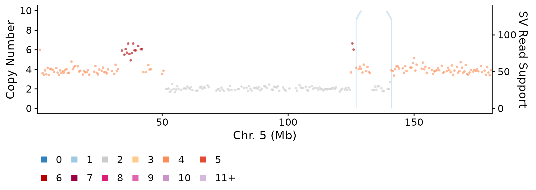
The vertical line marks each breakend and the arc joins them. Height
encodes read_count against the secondary axis on the
right.
Two styles
sv_style controls how SVs are drawn.
"curves" (the default) draws bezier curves coloured by
rearrangement_type; "lines_and_arcs" draws the
lines and arcs above, coloured by strand orientation.
"both" draws each.
plotCNprofile(cn, cellid = cell, chrfilt = "5", maxCN = 10,
              SV = sv_chr5, sv_style = "curves")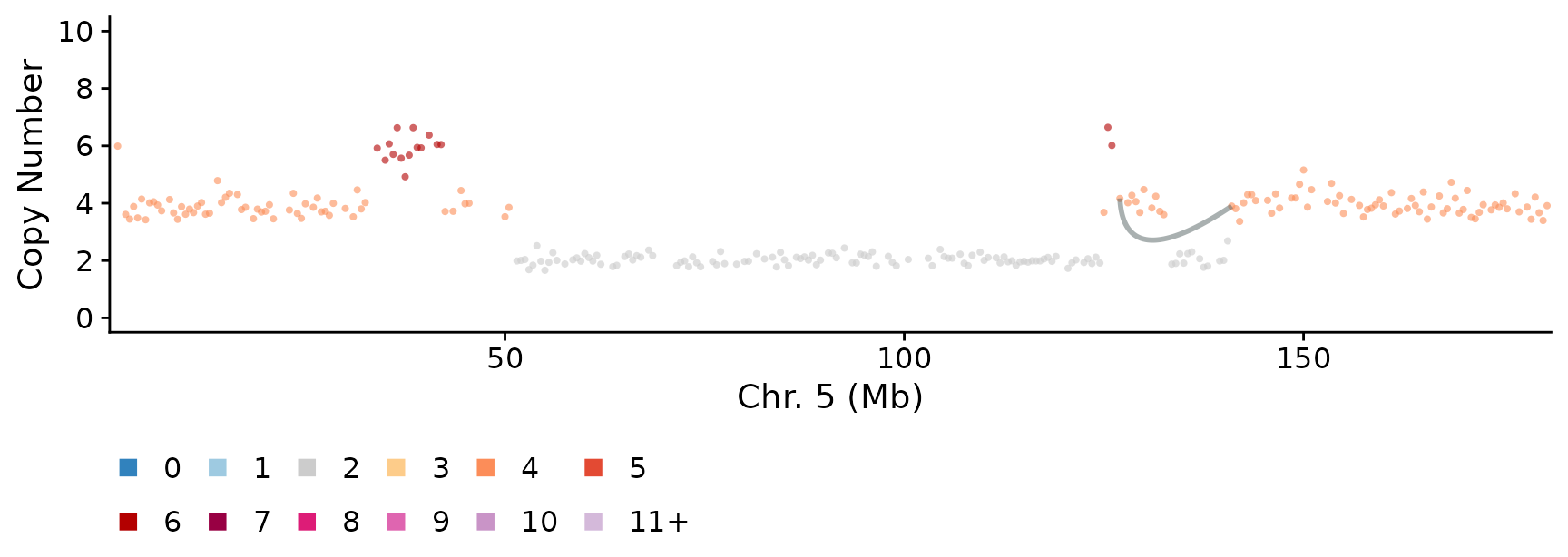
Many SVs
With a whole chromosome’s worth of SVs the picture degrades quickly. Chromosome 1 is the most rearranged in this sample:
sv_chr1 <- SVs %>% filter(chromosome_1 == "1", chromosome_2 == "1")
nrow(sv_chr1)
#> [1] 38

plotCNprofile(cn, cellid = cell, chrfilt = "1", maxCN = 10,
              SV = sv_chr1, sv_style = "lines_and_arcs")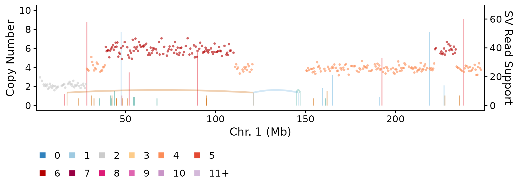
Two problems: the arcs sit on top of the copy number points, and because each arc’s height comes from its read count, every arc peaks somewhere different.
Moving the arcs into their own band
sv_arcs_above = TRUE draws the arcs in a band above the
copy number panel instead. Read count no longer affects the geometry, so
the secondary axis is dropped.
plotCNprofile(cn, cellid = cell, chrfilt = "1", maxCN = 10,
              SV = sv_chr1, sv_style = "lines_and_arcs",
              sv_arcs_above = TRUE)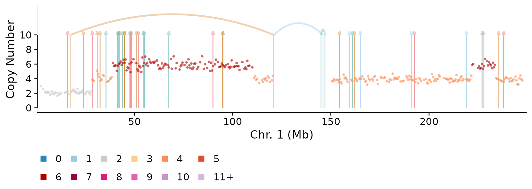
The copy number track is now unobstructed. sv_band_frac
sets how much of the panel the band takes:
plotCNprofile(cn, cellid = cell, chrfilt = "1", maxCN = 10,
              SV = sv_chr1, sv_style = "lines_and_arcs",
              sv_arcs_above = TRUE, sv_band_frac = 0.4)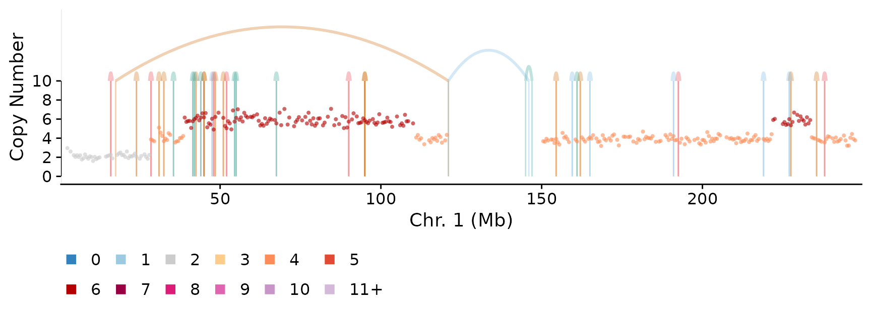
Arc height
By default the apex of each arc scales with the distance it spans, so
local rearrangements stay low and long-range ones arch over them.
sv_arc_scale = "fixed" gives every arc the same height
instead, which makes short SVs into narrow spikes:
plotCNprofile(cn, cellid = cell, chrfilt = "1", maxCN = 10,
              SV = sv_chr1, sv_style = "lines_and_arcs",
              sv_arcs_above = TRUE, sv_arc_scale = "fixed")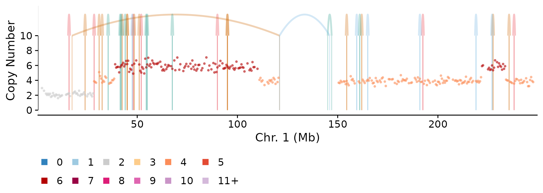
Two floors keep small SVs visible. sv_arc_min_width
matters most: an SV whose breakends fall in the same bin has zero width
and would not render at all — which at 500kb bins is every foldback.
sv_arc_min_height sets the apex of the shortest arcs.
plotCNprofile(cn, cellid = cell, chrfilt = "1", maxCN = 10,
              SV = sv_chr1, sv_style = "lines_and_arcs",
              sv_arcs_above = TRUE,
              sv_arc_min_height = 0.5, sv_arc_min_width = 0.01)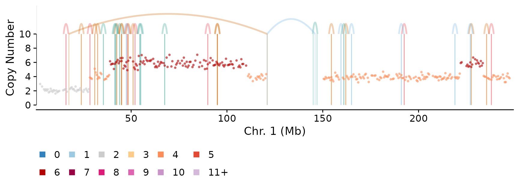
Splitting the band by copy number effect
sv_arc_side puts the baseline in the middle of the band
and splits arcs either side of it. With "cn_effect",
gain-associated junctions (tandem duplications, foldbacks,
translocations) arch up and loss-associated or copy-number-neutral ones
hang down, so an arc’s side predicts the copy number step beneath
it.
plotCNprofile(cn, cellid = cell, chrfilt = "1", maxCN = 10,
              SV = sv_chr1, sv_style = "lines_and_arcs",
              sv_arcs_above = TRUE, sv_band_frac = 0.4,
              sv_arc_side = "cn_effect")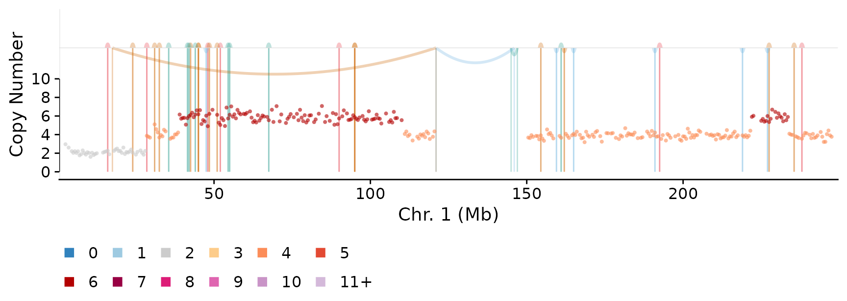
"translocation" and "foldback" are the
other built-in rules. You can also pass the name of a column in
SV holding "up"/"down" to split
on anything you like:
sv_chr1_side <- sv_chr1 %>%
  mutate(side = ifelse(read_count >= 30, "up", "down"))

plotCNprofile(cn, cellid = cell, chrfilt = "1", maxCN = 10,
              SV = sv_chr1_side, sv_style = "lines_and_arcs",
              sv_arcs_above = TRUE, sv_band_frac = 0.4,
              sv_arc_side = "side")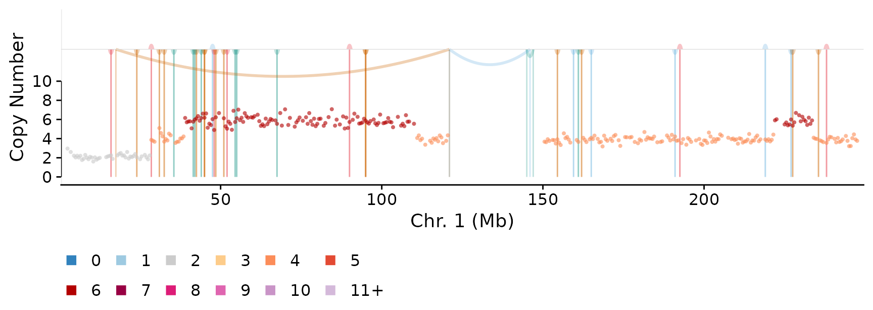
Breakpoint lines
The vertical lines run from 0 up to the arc baseline and are drawn
behind the copy number points. At high SV density they can dominate;
sv_show_lines = FALSE leaves the arcs alone.
plotCNprofile(cn, cellid = cell, chrfilt = "1", maxCN = 10,
              SV = sv_chr1, sv_style = "lines_and_arcs",
              sv_arcs_above = TRUE, sv_show_lines = FALSE)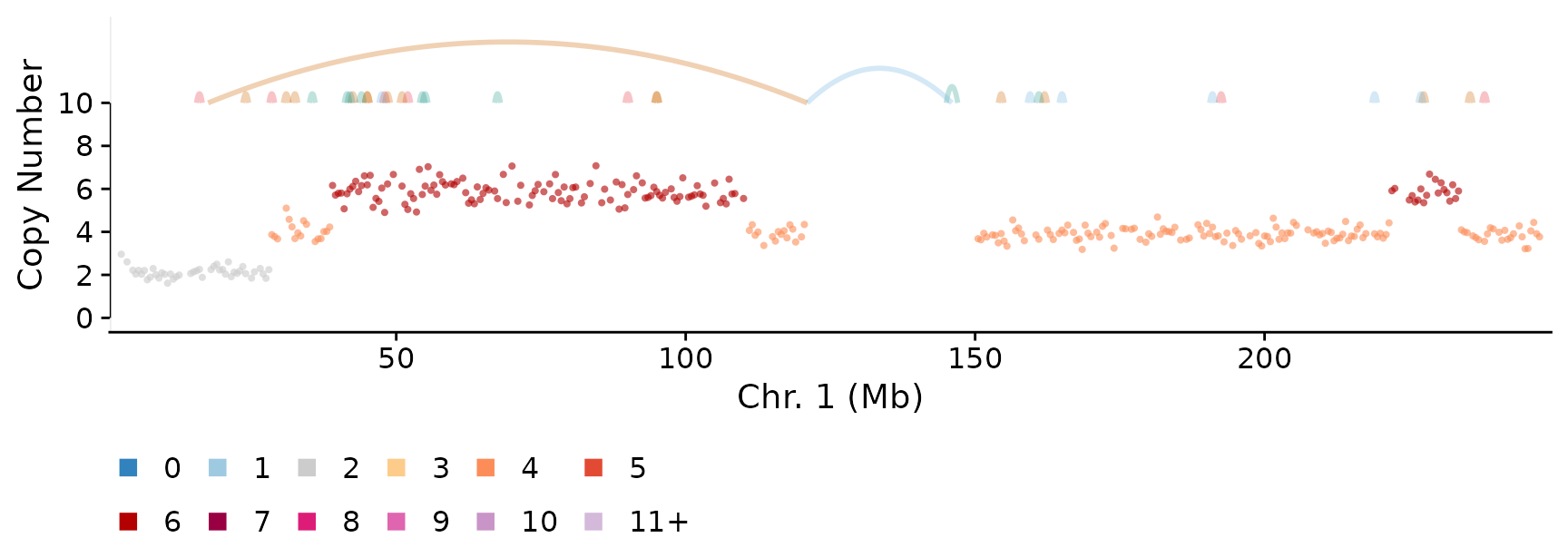
sv_line_alpha controls the lines independently of
sv_arc_alpha, which is useful because the lines sit behind
the data and can take more weight than the arcs.
Translocations
A translocation is only drawn when both breakends
are inside the plotted region, so inter-chromosomal SVs need both
chromosomes in view. Passing several chromosomes to chrfilt
works, but regions is usually better: it crops to the
interesting windows and keeps the arcs between them.
regions <- data.frame(chr = c("17", "2"), start = c(60, 5), end = c(70, 50))

sv_1702 <- SVs %>%
  filter((chromosome_1 == "17" & chromosome_2 == "2") |
         (chromosome_1 == "2"  & chromosome_2 == "17"))

plotCNprofile(cn, cellid = cell, regions = regions, maxCN = 10,
              SV = sv_1702, sv_style = "lines_and_arcs",
              sv_arcs_above = TRUE, sv_band_frac = 0.35)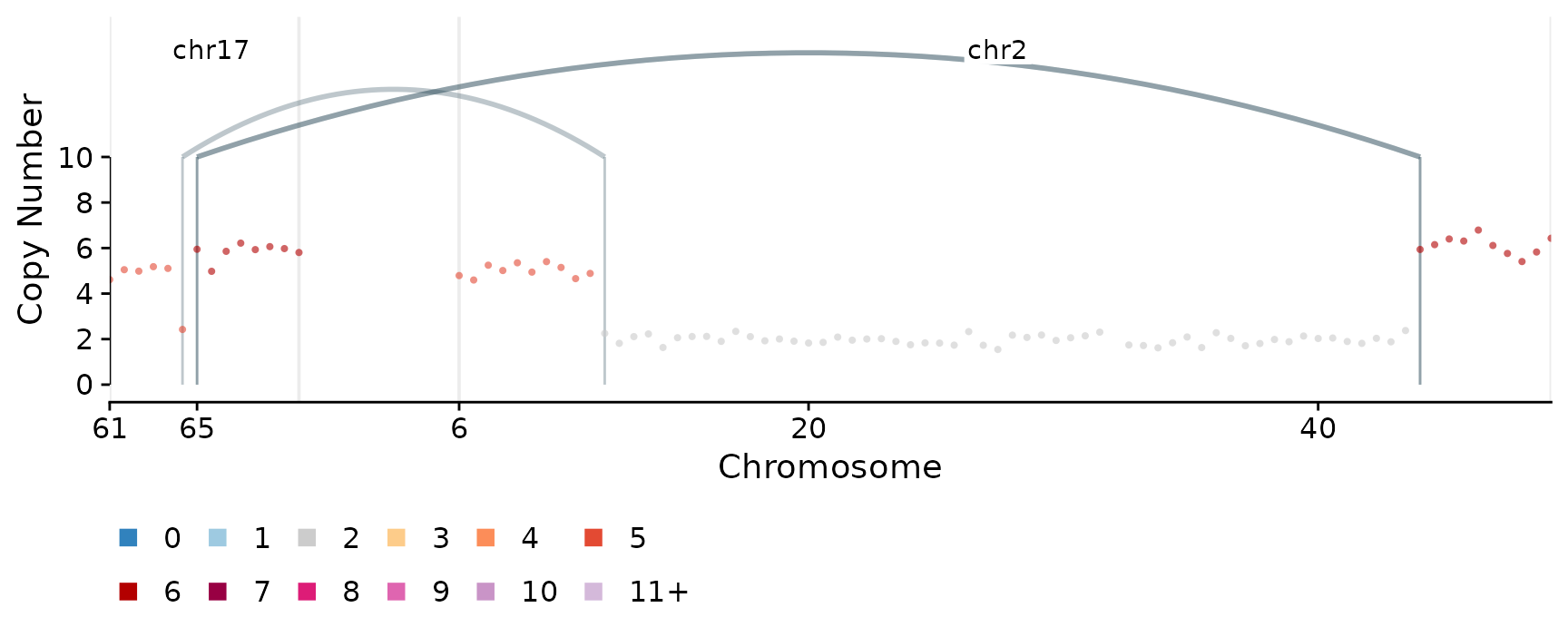
show_chrbreaks = FALSE removes the grey lines that
bracket each region, and ybreaks overrides the y axis
breaks — useful in short panels, where the defaults collide.
plotCNprofile(cn, cellid = cell, regions = regions, maxCN = 10,
              SV = sv_1702, sv_style = "lines_and_arcs",
              sv_arcs_above = TRUE, sv_band_frac = 0.35,
              show_chrbreaks = FALSE, ybreaks = c(0, 5, 10))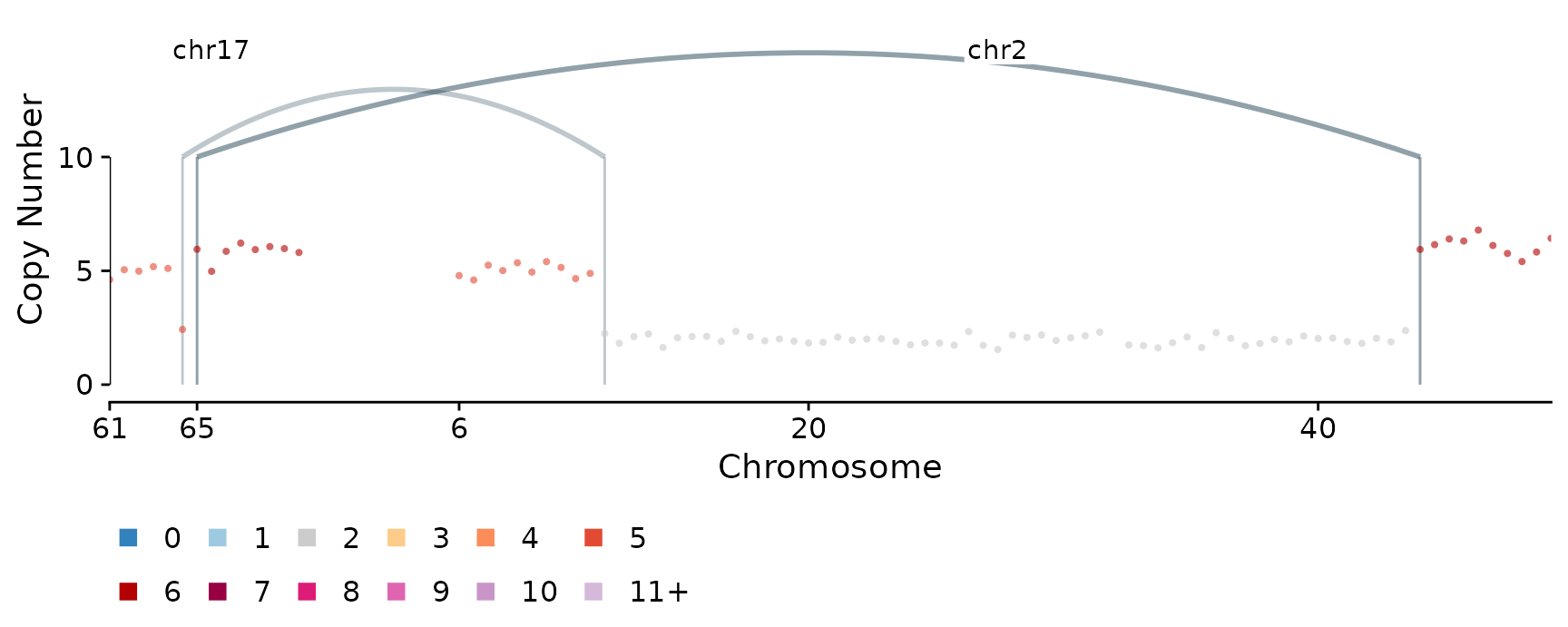
Whole genome
Everything works genome-wide, though at this scale only the broadest structure is legible.
plotCNprofile(cn, cellid = cell, maxCN = 10,
              SV = SVs, sv_style = "lines_and_arcs",
              sv_arcs_above = TRUE, sv_band_frac = 0.3,
              sv_show_lines = FALSE, sv_arc_alpha = 0.6)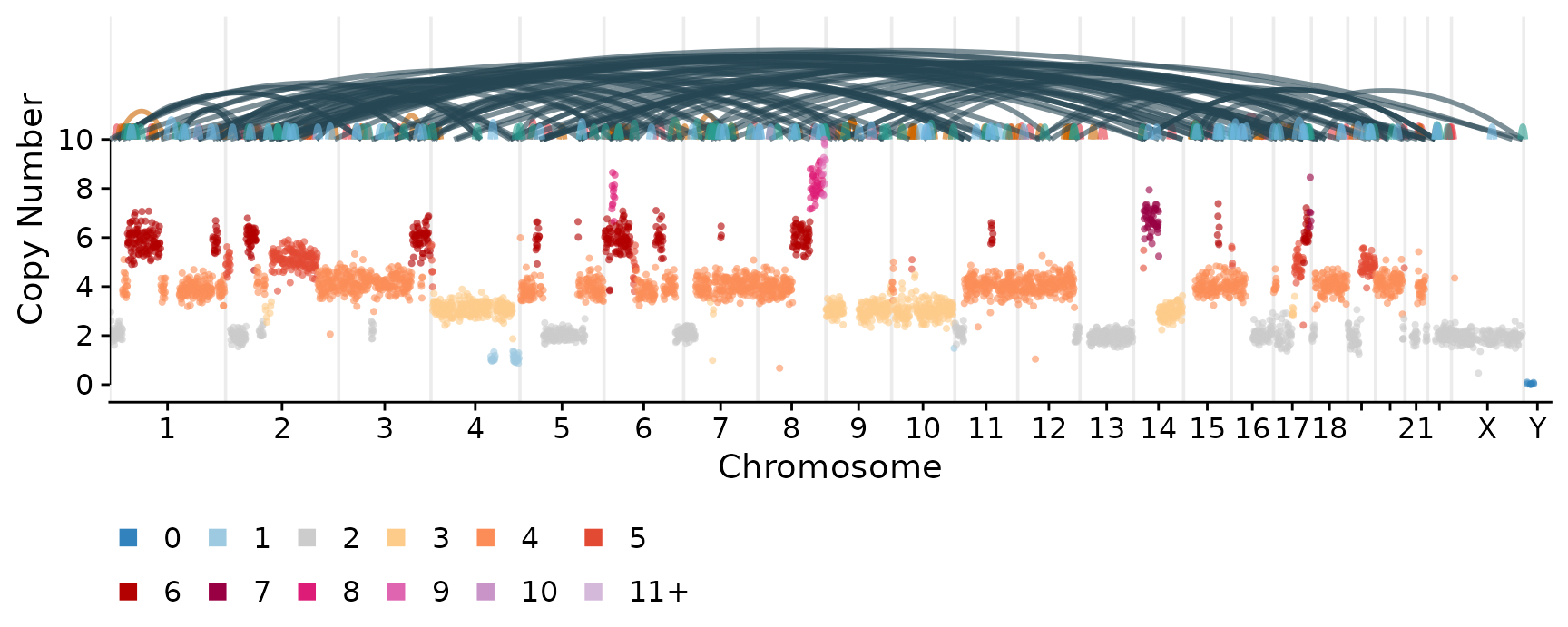
Legend
Orientation colours are off by default.
show_sv_legend = TRUE adds them to the plot, or
get_sv_lines_and_arcs_legend() returns a standalone legend
for assembling figures by hand.
cowplot::plot_grid(get_sv_lines_and_arcs_legend(direction = "horizontal"))