---
title: "Figure 1 -- cohort overview"
author: "Matthew Zatzman"
execute:
warning: false
error: false
format:
html:
code-fold: true
code-tools: true
toc: true
toc-depth: 3
---
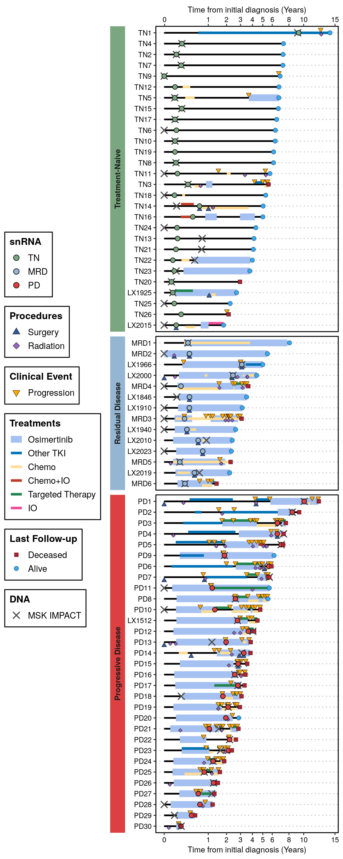
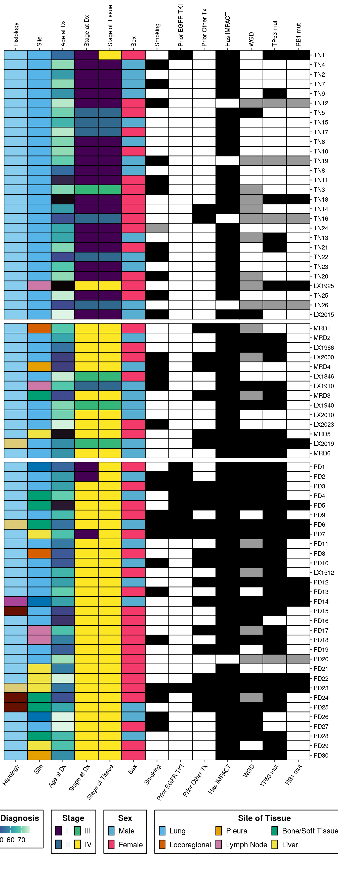
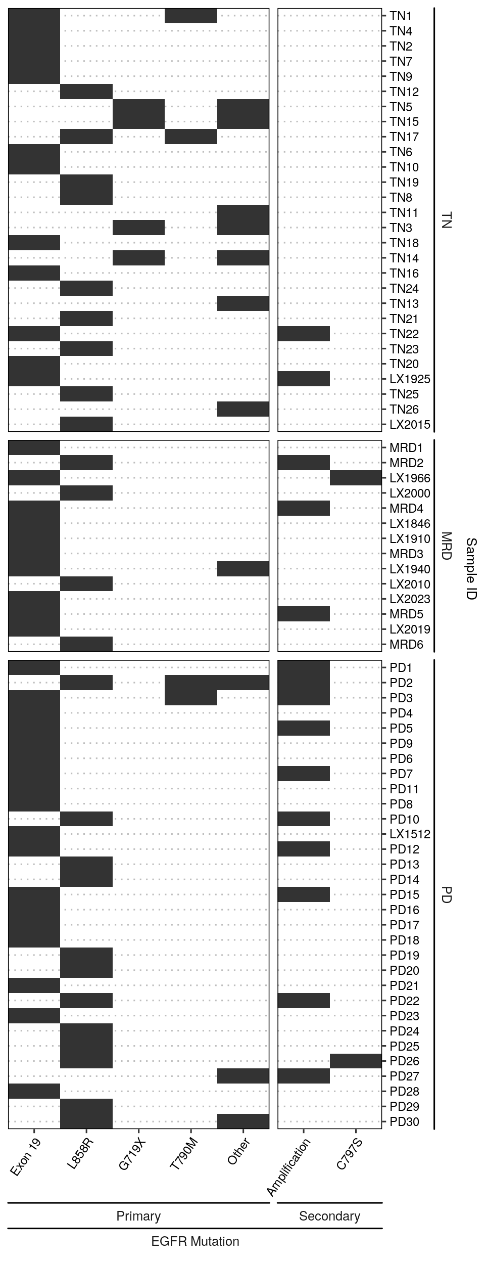
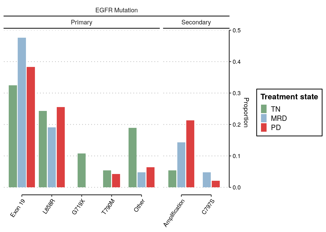
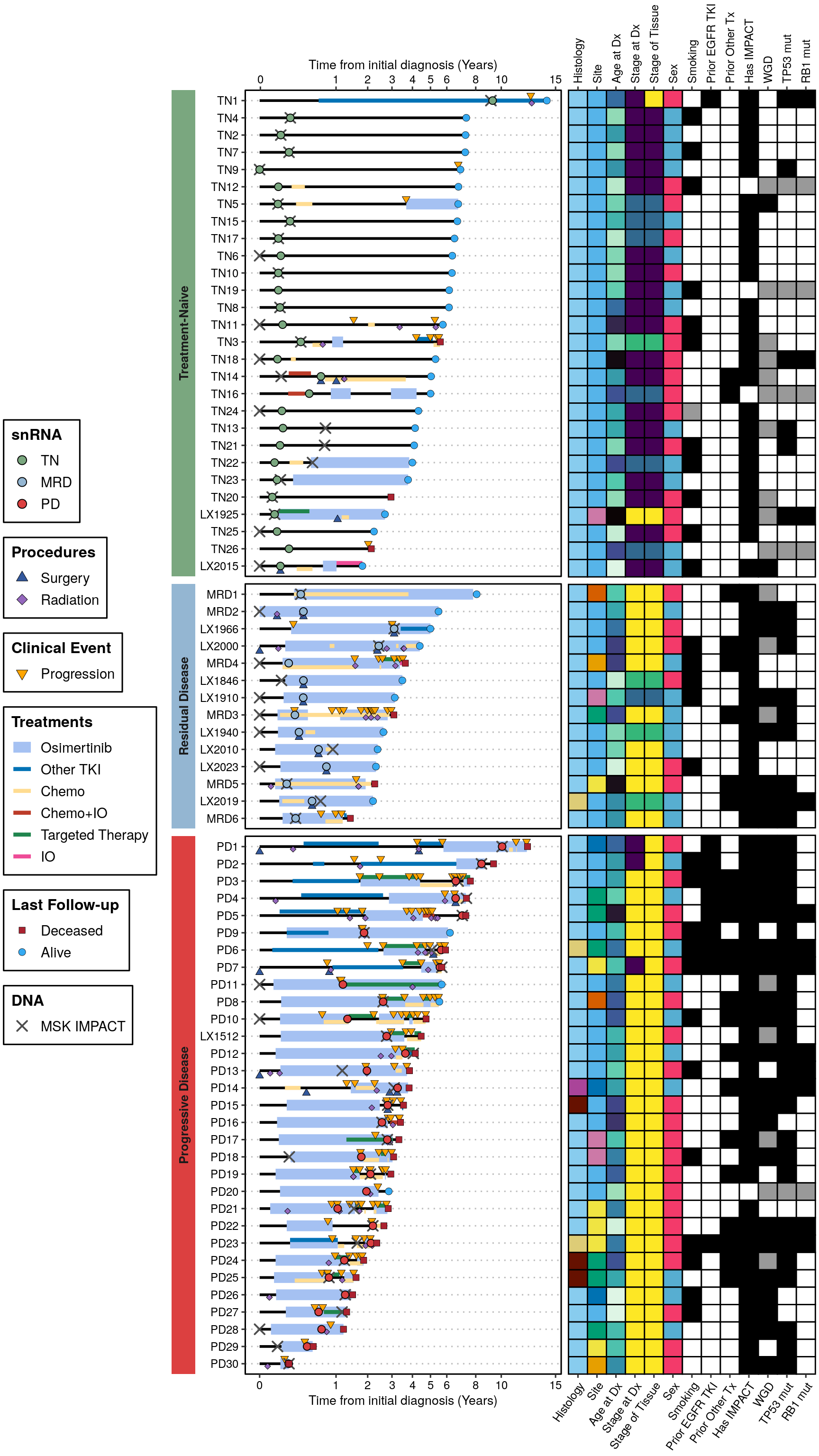
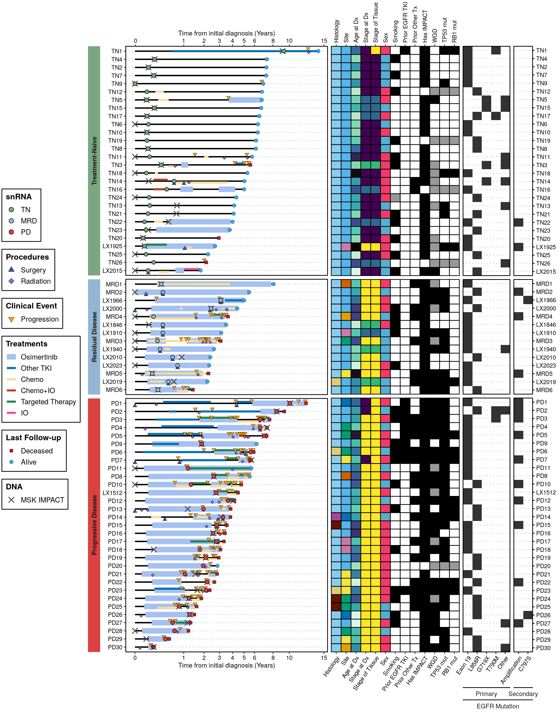
Reproduces the Figure 1 cohort panels -- the swimmer plot, the patient-level
annotation tiles and the EGFR variant summary -- from two files in `paper_data/`:
- **`supplemental_tables.xlsx`**, sheet `Table S1 - Cohort Metadata`. The published
cohort table: one row per specimen, and one specimen per patient, so it is also the
patient-level table this figure needs. The annotation tiles, the *EGFR* variant
summary and the osimertinib timing are all derived from it below.
- **`patient_event_timeline.csv`**. The clinical event timeline -- diagnosis, treatment
intervals, progression, surgery, radiation, sample collection and MSK-IMPACT
sequencing -- as day offsets from each patient's initial diagnosis. No published table
carries it, so it is deposited alongside them.
Run `00_download_convert.qmd` first to build `paper_data/`.
```{r setup}
#| output: false
# Same set the source notebook attaches, in the same order.
library(tidyverse)
library(here)
library(ggsci)
library(ggthemes)
library(glue)
library(patchwork)
library(cowplot)
library(ggnewscale)
library(ggh4x)
library(ggtext)
devtools::load_all(here())
colors <- load_colors()

dir.create(here("plots"), showWarnings = FALSE)
```
```{r load-data}
s1 <- readxl::read_excel(here("paper_data", "supplemental_tables.xlsx"),
                         sheet = "Table S1 - Cohort Metadata")

timeline <- readr::read_csv(here("paper_data", "patient_event_timeline.csv"),
                            show_col_types = FALSE)

stopifnot(
  nrow(s1) == 73L,
  !anyDuplicated(s1$sample_id),
  setequal(timeline$patient_id, s1$sample_id)
)

# Table S1 is a spreadsheet: missing values arrive as the literal string "NA", and one of
# those makes the whole column character however numeric or logical the rest of it is.
# as.numeric() / as.logical() map both that string and a real NA to NA.
as_num <- function(x) suppressWarnings(as.numeric(as.character(x)))
as_flag <- function(x) as.logical(as.character(x))
```
# Prepare Patient-Level Data
One row per patient, for the swimmers plot y-axis.
```{r}
# One timepoint per patient, so the facet group is just that timepoint. The published
# figure has a fourth "Pairs" facet for a patient whose second specimen was
# single-cell rather than single-nucleus and is not in the deposit.
patient_timepoints <- s1 %>%
  distinct(patient_id = sample_id, time_point) %>%
  group_by(patient_id) %>%
  summarise(
    n_timepoints = n_distinct(time_point),
    facet_group = paste(sort(unique(time_point)), collapse = "+"),
    .groups = "drop"
  )

stopifnot(all(patient_timepoints$n_timepoints == 1L))

# Patient-level info for the swimmer lanes and the annotation tiles
patient_info <- s1 %>%
  transmute(
    patient_id = sample_id,
    gender = sex,
    smoking = na_if(smoking_history_simple, "NA"),
    smoking_yn = case_when(
      smoking == "Never Smoker" ~ "No",
      smoking %in% c("Former Smoker", "Current Smoker") ~ "Yes",
      .default = NA_character_
    ),
    stage_dx = stage_at_initial_diagnosis_simple,
    stage_dx_tnm = stage_at_initial_diagnosis,
    age = as_num(age_at_intial_diagnosis),
    histology = histology_predominant_short,
    prior_egfr_tki = as_flag(prior_tki),
    prior_non_egfr_targeted = as_flag(prior_non_egfr_targeted),
    prior_other_therapy = as_flag(prior_therapy),
    site = site_of_tissue_simple,
    stage_of_tissue_simple,
    has_impact = as_flag(has_impact),
    tp53mut = as_flag(tp53mut),
    rb1_mut = as_flag(rb1mut),
    facets_wgd = as_flag(facets_wgd)
  ) %>%
  left_join(patient_timepoints, by = "patient_id")
```
# Build Timeline Components
## Diagnosis and follow-up endpoints
```{r}
# Diagnosis day is always 0
dx_events <- timeline %>%
  filter(event_type == "Diagnosis") %>%
  select(patient_id, dx_day = start_day)

# Last contact / death = endpoint of the swimmer bar
endpoint_events <- timeline %>%
  filter(event_type %in% c("Last Contact", "Death")) %>%
  group_by(patient_id) %>%
  slice_max(start_day, n = 1) %>%
  ungroup() %>%
  select(patient_id, last_day = start_day, endpoint_type = event_type)

# Combine into swimmers base
swimmers_base <- patient_info %>%
  left_join(dx_events, by = "patient_id") %>%
  left_join(endpoint_events, by = "patient_id") %>%
  mutate(
    dx_day = replace_na(dx_day, 0),
    # Convert days to years
    last_yr = last_day / 365.25,
    dx_yr = dx_day / 365.25
  )

swimmers_base$facet_group <- factor(
  swimmers_base$facet_group,
  levels = c("TN", "MRD", "PD")
)
```
## Treatments
```{r}
treatments <- timeline %>%
  filter(event_type == "Treatment", !is.na(start_day)) %>%
  select(patient_id, event_subtype, event_detail, start_day, end_day) %>%
  mutate(
    # Simplify treatment categories
    treatment_cat = case_when(
      event_detail == "osimertinib" ~ "Osimertinib",
      event_subtype == "EGFR TKI" ~ "Other TKI",
      event_subtype == "Chemotherapy" ~ "Chemo",
      event_subtype == "Targeted Therapy" ~ "Targeted Therapy",
      event_subtype == "Anti-angiogenic" ~ "Chemo",
      event_subtype == "Immunotherapy" ~ "IO",
      .default = "Other"
    ),
    start_yr = start_day / 365.25,
    end_yr = end_day / 365.25
  )

# Detect Chemo+IO via temporal overlap (segment-level, not patient-level)
# Only reclassify the specific Chemo/IO segments that actually overlap each other
chemo_segs <- treatments %>%
  filter(treatment_cat == "Chemo") %>%
  mutate(row_id = row_number()) %>%
  select(patient_id, row_id, c_start = start_day, c_end = end_day)
io_segs <- treatments %>%
  filter(treatment_cat == "IO") %>%
  mutate(row_id = row_number()) %>%
  select(patient_id, row_id, i_start = start_day, i_end = end_day)

overlap_pairs <- inner_join(chemo_segs, io_segs, by = "patient_id",
                            relationship = "many-to-many") %>%
  filter(c_start <= coalesce(i_end, i_start) & i_start <= coalesce(c_end, c_start))

# Mark only overlapping segments
chemo_overlap_idx <- which(
  treatments$treatment_cat == "Chemo" &
  seq_len(nrow(treatments)) %in% (
    treatments %>%
      mutate(.row = row_number()) %>%
      filter(treatment_cat == "Chemo") %>%
      mutate(row_id = row_number()) %>%
      filter(row_id %in% overlap_pairs$row_id.x) %>%
      pull(.row)
  )
)
io_overlap_idx <- which(
  treatments$treatment_cat == "IO" &
  seq_len(nrow(treatments)) %in% (
    treatments %>%
      mutate(.row = row_number()) %>%
      filter(treatment_cat == "IO") %>%
      mutate(row_id = row_number()) %>%
      filter(row_id %in% overlap_pairs$row_id.y) %>%
      pull(.row)
  )
)

treatments$treatment_cat[c(chemo_overlap_idx, io_overlap_idx)] <- "Chemo+IO"

# Deduplicate into treatment episodes
# Segments of the same category within 90 days of each other are merged into one episode;
# segments separated by >90 days remain as distinct bars
min_segment_width_yr <- 15 / 365.25  # minimum visible width
episode_gap_days <- 90

treatments_dedup <- treatments %>%
  arrange(patient_id, treatment_cat, start_day) %>%
  group_by(patient_id, treatment_cat) %>%
  mutate(
    prev_end = lag(as.numeric(end_day), default = -Inf),
    gap = as.numeric(start_day) - prev_end,
    episode = cumsum(replace_na(gap > episode_gap_days, TRUE))
  ) %>%
  group_by(patient_id, treatment_cat, episode) %>%
  summarise(
    start_yr = min(start_yr, na.rm = TRUE),
    end_yr = max(end_yr, na.rm = TRUE),
    detail = paste(unique(event_detail), collapse = " + "),
    .groups = "drop"
  ) %>%
  mutate(
    zero_duration = is.na(end_yr) | (end_yr - start_yr) < min_segment_width_yr,
    end_yr = if_else(zero_duration, start_yr + min_segment_width_yr, end_yr)
  )

# Separate osimertinib from other treatments for layering
osi_df <- treatments_dedup %>% filter(treatment_cat == "Osimertinib")
other_tx_df <- treatments_dedup %>% filter(treatment_cat != "Osimertinib")
```
## Events: Progression, Surgery, Radiation, Sample Collection
```{r}
progressions <- timeline %>%
  filter(event_type == "Progression") %>%
  mutate(event_yr = start_day / 365.25) %>%
  select(patient_id, event_yr, event_detail)

surgeries <- timeline %>%
  filter(event_type == "Surgery", !is.na(start_day)) %>%
  mutate(event_yr = start_day / 365.25) %>%
  select(patient_id, event_yr, event_detail = event_subtype)

radiation <- timeline %>%
  filter(event_type == "Radiation", !is.na(start_day)) %>%
  mutate(event_yr = start_day / 365.25) %>%
  select(patient_id, event_yr, event_detail = event_subtype)

# One collection event per specimen
sample_collections <- timeline %>%
  filter(event_type == "Sample Collection", !is.na(start_day)) %>%
  mutate(
    event_yr = start_day / 365.25,
    timepoint = event_subtype
  ) %>%
  select(patient_id, event_yr, timepoint)

stopifnot(nrow(sample_collections) == 73L)

# MSK-IMPACT sequencing travels as timeline rows like any other event type
impact_seq_matched <- timeline %>%
  filter(event_type == "IMPACT Sequencing") %>%
  mutate(event_yr = start_day / 365.25) %>%
  select(patient_id, event_yr)

stopifnot(nrow(impact_seq_matched) == 68L,
          !anyDuplicated(impact_seq_matched$patient_id))
```
Time from osimertinib start to sample collection.
```{r}
osi_to_sc <- s1 %>%
  transmute(
    patient_id = sample_id,
    timepoint = time_point,
    days_from_osi = as_num(days_from_first_osi),
    cumulative_osi_days = as_num(days_osi_at_collection)
  ) %>%
  filter(!is.na(days_from_osi))

stopifnot(nrow(osi_to_sc) == 53L)

osi_to_sc %>%
  group_by(timepoint) %>%
  summarize(
    mean_days_from_osi = mean(days_from_osi, na.rm = TRUE),
    median_days_from_osi = median(days_from_osi, na.rm = TRUE),
    days_from_osi_iqr = paste(quantile(days_from_osi, c(0.25, 0.75), na.rm = TRUE), collapse = ", "),
    range_days_from_osi = paste(range(days_from_osi, na.rm = TRUE), collapse = ", "),
    mean_cumulative_osi = mean(cumulative_osi_days, na.rm = TRUE),
    median_cumulative_osi = median(cumulative_osi_days, na.rm = TRUE),
    cumulative_osi_iqr = paste(quantile(cumulative_osi_days, c(0.25, 0.75), na.rm = TRUE), collapse = ", "),
    range_cumulative_osi = paste(range(cumulative_osi_days, na.rm = TRUE), collapse = ", ")
  )
```
# Swimmers Plot
## Main Panel
```{r, fig.width = 6, fig.height = 15}
# SETTINGS
tri_stroke <- 0.25
tri_size <- 2
tri_nudge <- 0.3

# Facet relabeller
facet_names <- c(
  "TN" = "Treatment-Naive",
  "MRD" = "Residual Disease",
  "PD" = "Progressive Disease",
  "Paired" = "Pairs"
)

# Backgrounds for each facet
backgrounds <- list(
  element_rect(fill = colors$time_point[["TN"]], color = "black", linewidth = 1),
  element_rect(fill = colors$time_point[["MRD"]], color = NA),
  element_rect(fill = colors$time_point[["PD"]], color = NA),
  element_rect(fill = "#c9a0dc", color = NA)
)

# Merge swimmers_base with treatment data for plotting
# Need patient_id on y axis, ordered by last_yr within facet groups
plot_base <- swimmers_base %>%
  mutate(patient_id = fct_reorder(patient_id, last_yr, .fun = max))

# Join treatments to get facet info
osi_plot <- osi_df %>%
  left_join(swimmers_base %>% select(patient_id, facet_group), by = "patient_id")
other_tx_plot <- other_tx_df %>%
  left_join(swimmers_base %>% select(patient_id, facet_group), by = "patient_id")

# Join events to get facet info
prog_plot <- progressions %>%
  left_join(swimmers_base %>% select(patient_id, facet_group), by = "patient_id")
surg_plot <- surgeries %>%
  left_join(swimmers_base %>% select(patient_id, facet_group), by = "patient_id")
rad_plot <- radiation %>%
  left_join(swimmers_base %>% select(patient_id, facet_group), by = "patient_id")
sc_plot <- sample_collections %>%
  left_join(swimmers_base %>% select(patient_id, facet_group), by = "patient_id")
impact_seq_plot <- impact_seq_matched %>%
  left_join(swimmers_base %>% select(patient_id, facet_group, last_yr), by = "patient_id") %>%
  filter(!is.na(facet_group))

swimmers_plot <- plot_base %>%
  ggplot(aes(y = patient_id)) +
  # --- BASELINE: Diagnosis to last follow-up ---
  geom_segment(aes(x = dx_yr, xend = last_yr), linewidth = 1, color = "black") +
  # --- OSIMERTINIB INTERVALS ---
  geom_segment(
    data = osi_plot, linewidth = 4,
    aes(x = start_yr, xend = end_yr, color = "Osimertinib"),
    position = position_nudge(y = 0)
  ) +
  # --- OTHER TREATMENTS (dodged so overlapping categories are visible) ---
  geom_segment(
    data = other_tx_plot, linewidth = 1.5,
    aes(x = start_yr, xend = end_yr, color = treatment_cat, group = treatment_cat),
    position = position_dodge(width = 0.7)
  ) +
  scale_color_manual(
    na.translate = FALSE,
    name = "Treatments",
    values = c(
      "Osimertinib" = "#a5c1f2",
      "Other TKI" = "#0072B5FF",
      "Chemo" = "#FFDC91FF",
      "Chemo+IO" = "#BC3C29FF",
      "Targeted Therapy" = "#20854EFF",
      "IO" = "#EE4C97FF",
      "Other" = "#8B919C"
    ),
    limits = c("Osimertinib", "Other TKI", "Chemo", "Chemo+IO", "Targeted Therapy", "IO"),
    guide = guide_legend(order = 4)
  ) +
  # --- EVENTS: Progression ---
  geom_point(
    data = prog_plot,
    aes(x = event_yr, fill = "Progression"),
    size = tri_size, stroke = tri_stroke,
    position = position_nudge(y = tri_nudge), pch = 25
  ) +
  scale_fill_manual(
    name = "Clinical Event",
    values = c("Progression" = "orange"),
    guide = guide_legend(override.aes = list(size = 3), order = 3),
    limits = c("Progression")
  ) +
  new_scale_fill() +
  # --- EVENTS: Surgery ---
  geom_point(
    data = surg_plot,
    aes(x = event_yr, fill = "Surgery"),
    size = tri_size, stroke = tri_stroke,
    position = position_nudge(y = -tri_nudge), pch = 24
  ) +
  # --- EVENTS: Radiation ---
  geom_point(
    data = rad_plot,
    aes(x = event_yr, fill = "Radiation"),
    size = tri_size * 0.8, stroke = tri_stroke,
    position = position_nudge(y = -tri_nudge * 0.5), pch = 23
  ) +
  scale_fill_manual(
    name = "Procedures",
    values = c(
      "Surgery" = "#33589c",
      "Radiation" = "#9467bd"
    ),
    guide = guide_legend(override.aes = list(size = 3), order = 2),
    limits = c("Surgery", "Radiation")
  ) +
  new_scale_fill() +
  # --- IMPACT SEQUENCING ---
  geom_point(
    data = impact_seq_plot,
    aes(x = event_yr, shape = "MSK IMPACT"),
    size = 3, stroke = 1, color = "grey30"
  ) +
  scale_shape_manual(
    name = "DNA",
    values = c("MSK IMPACT" = 4),
    guide = guide_legend(order = 6)
  ) +
  new_scale("shape") +
  new_scale_fill() +
  # --- SAMPLE COLLECTION ---
  geom_point(
    data = sc_plot,
    aes(x = event_yr, fill = timepoint),
    size = tri_size + 0.5, stroke = 0.5, pch = 21,
    position = position_nudge(y = 0)
  ) +
  scale_fill_manual(
    name = "snRNA",
    values = c(
      "TN" = colors$time_point[["TN"]],
      "MRD" = colors$time_point[["MRD"]],
      "PD" = colors$time_point[["PD"]]
    ),
    limits = c("TN", "MRD", "PD"),
    # labels = c("TN" = "Treatment-Naive", "MRD" = "Residual Disease", "PD" = "Progressive Disease"),
    guide = guide_legend(override.aes = list(size = 3, pch = 21), order = 1)
  ) +
  new_scale_fill() +
  # --- LAST STATUS (Alive/Deceased) ---
  geom_point(
    aes(x = last_yr, shape = endpoint_type, fill = endpoint_type),
    size = 2.5, stroke = 0.2
  ) +
  scale_shape_manual(
    name = "Last Follow-up",
    values = c("Last Contact" = 21, "Death" = 22),
    labels = c("Last Contact" = "Alive", "Death" = "Deceased"),
    guide = guide_legend(order = 5)
  ) +
  scale_fill_manual(
    name = "Last Follow-up",
    values = c("Last Contact" = "#35aaf2", "Death" = "#ab2230"),
    labels = c("Last Contact" = "Alive", "Death" = "Deceased"),
    guide = guide_legend(order = 5)
  ) +
  new_scale_fill() +
  new_scale("shape") +
  # --- AXIS ---
  labs(x = "Time from initial diagnosis (Years)", y = NULL) +
  scale_x_sqrt(
    breaks = c(0, 1, 2, 3, 4, 5, 6, 8, 10, 15, 20, 25, 30),
    labels = c(0, 1, 2, 3, 4, 5, 6, 8, 10, 15, 20, 25, 30),
    sec.axis = sec_axis(~.,
      name = "Time from initial diagnosis (Years)",
      breaks = c(1e-4, 1, 2, 3, 4, 5, 6, 8, 10, 15, 20, 25, 30),
      labels = c(0, 1, 2, 3, 4, 5, 6, 8, 10, 15, 20, 25, 30)
    )
  ) +
  # --- FACET ---
  facet_grid2(facet_group ~ .,
    scales = "free", space = "free_y", switch = "y",
    strip = strip_themed(
      background_y = backgrounds,
      text_y = list(
        element_text(face = "bold"),
        element_text(face = "bold"),
        element_text(face = "bold"),
        element_text(face = "bold")
      ),
      clip = "off"
    ),
    labeller = as_labeller(facet_names)
  ) +
  theme_clean() +
  theme(
    panel.border = element_part_rect(side = "tblr", fill = NA),
    axis.line.x = element_blank(),
    axis.line.y = element_blank(),
    plot.background = element_blank(),
    strip.placement = "outside",
    strip.clip = "off",
    legend.position = "left"
  ) +
  coord_cartesian(clip = "off")

swimmers_plot
```
## Side Annotations
```{r, fig.width = 7, fig.height = 18}
anno_data <- swimmers_base %>%
  mutate(
    patient_id = fct_reorder(patient_id, last_yr, .fun = max),
    smoking_simple = case_when(
      smoking_yn == "Yes" ~ TRUE,
      smoking_yn == "No" ~ FALSE,
      .default = NA
    ),
    # Collapse prior non-EGFR targeted + prior other therapy into one column
    prior_other_systemic = prior_non_egfr_targeted | prior_other_therapy,
    # `Site_of_Tissue_Standardized` already arrives in the canonical seven-level
    # space shared with Table S1 and Figure 2C, so it is only releveled here.
    # It used to be passed through an fct_recode() that renamed Pleura ->
    # "Pleural effusion"; that name is not in the palette, so the level fell
    # through to na.value and vanished from the key. Do not reintroduce it.
    site = factor(site, levels = names(colors$site_of_tissue_simple))
  )

# The Site of Tissue key must carry all seven levels, in palette order.
stopifnot(setdiff(unique(as.character(anno_data$site)), NA) %in%
            names(colors$site_of_tissue_simple))

meta_plot <- anno_data %>%
  ggplot(aes(y = patient_id)) +
  # Age
  geom_tile(aes(x = "Age at Dx", fill = age), color = "black", linewidth = 0.5) +
  scale_fill_gradientn(
    name = "Age at Diagnosis",
    colours = viridis::mako(10),
    guide = guide_colorbar(order = 2, position = "bottom", keywidth = 5, keyheight = 0.7)
  ) +
  new_scale_fill() +
  # Histology
  geom_tile(aes(x = "Histology", fill = histology), color = "black", linewidth = 0.5) +
  scale_fill_manual(
    name = "Histology",
    values = c(
      colors$histology_predominant_short
    ),
    na.value = "grey80",
    guide = guide_legend(order = 1, position = "bottom", keywidth = 0.7, keyheight = 1, ncol = 2)
  ) +
  new_scale_fill() +
  # Stage of tissue (for the specific sample collected)
  geom_tile(aes(x = "Stage of Tissue", fill = stage_of_tissue_simple), color = "black", linewidth = 0.5) +
  # Stage at diagnosis
  geom_tile(aes(x = "Stage at Dx", fill = stage_dx), color = "black", linewidth = 0.5) +
  scale_fill_viridis_d(
    name = "Stage",
    guide = guide_legend(order = 3, position = "bottom", keywidth = 0.7, keyheight = 1, ncol = 2)
  ) +
  new_scale_fill() +
  geom_tile(aes(x = "Sex", fill = gender), color = "black", linewidth = 0.5) +
  scale_fill_manual(
    name = "Sex",
    values = colors$sex,
    breaks = names(colors$sex),
    na.value = "grey80",
    guide = guide_legend(order = 4, keywidth = 0.7, keyheight = 1, ncol = 1, position = "bottom")
  ) +
  new_scale_fill() +
  # Site of tissue
  geom_tile(aes(x = "Site", fill = site), color = "black", linewidth = 0.5) +
  scale_fill_manual(
    name = "Site of Tissue",
    values = colors$site_of_tissue_simple,
    breaks = names(colors$site_of_tissue_simple),
    na.value = "grey80",
    guide = guide_legend(order = 5, position = "bottom", keywidth = 0.7, keyheight = 1, nrow = 2)
  ) +
  new_scale_fill() +
  # All binary (Yes/No/NA) tiles: Smoking, Prior treatments, IMPACT annotations
  geom_tile(aes(x = "Smoking", fill = smoking_simple), color = "black", linewidth = 0.5) +
  geom_tile(aes(x = "Prior EGFR TKI", fill = prior_egfr_tki), color = "black", linewidth = 0.5) +
  geom_tile(aes(x = "Prior Other Tx", fill = prior_other_systemic), color = "black", linewidth = 0.5) +
  geom_tile(aes(x = "Has IMPACT", fill = has_impact), color = "black", linewidth = 0.5) +
  geom_tile(aes(x = "WGD", fill = facets_wgd), color = "black", linewidth = 0.5) +
  geom_tile(aes(x = "TP53 mut", fill = tp53mut), color = "black", linewidth = 0.5) +
  geom_tile(aes(x = "RB1 mut", fill = rb1_mut), color = "black", linewidth = 0.5) +
  scale_fill_manual(
    name = "Yes / No / NA",
    values = colors$tf[c("TRUE", "FALSE")],
    labels = c("TRUE" = "Yes", "FALSE" = "No"),
    na.value = colors$tf[["NA"]],
    guide = guide_legend(order = 6, keywidth = 0.7, keyheight = 1, ncol = 1, position = "bottom")
  ) +
  # Facet
  facet_grid2(facet_group ~ ., scales = "free", space = "free_y") +
  scale_y_discrete(position = "right", expand = c(0, 0)) +
  scale_x_discrete(
    expand = c(0, 0),
    limits = c("Histology", "Site", "Age at Dx", "Stage at Dx", "Stage of Tissue", "Sex", "Smoking", "Prior EGFR TKI", "Prior Other Tx", "Has IMPACT", "WGD", "TP53 mut", "RB1 mut"),
    sec.axis = dup_axis()
  ) +
  guides(x = guide_axis(angle = 55), x.sec = guide_axis(angle = 90)) +
  labs(x = NULL, y = NULL) +
  theme_clean() +
  theme(
    strip.text.y = element_blank(),
    panel.border = element_blank(),
    plot.background = element_blank(),
    axis.line.x = element_blank(),
    axis.line.y = element_blank(),
    panel.grid.major.y = element_blank(),
    legend.key.height = unit(1, "lines"),
    legend.key.width = unit(0.6, "lines"),
    legend.title.position = "top",
    legend.title = element_text(hjust = 0.5)
  )

meta_plot
```
## EGFR mutations
```{r, fig.width = 5, fig.height = 13}
egfr_hits <- s1 %>%
  select(sample_id, egfr_primary, egfr_secondary, time_point) %>%
  pivot_longer(cols = c(egfr_primary, egfr_secondary),
               names_to = "variant_type", values_to = "variant") %>%
  filter(variant != "NA") %>%
  separate_longer_delim(variant, delim = ", ") %>%
  distinct() %>%
  mutate(
    egfr_cat = case_when(
      grepl("*74.*[ins|del]|exon 19 del|T751_I759", variant) ~ "Exon 19",
      grepl("G719*", variant) ~ "G719X",
      variant == "L858R" ~ "L858R",
      variant == "T790M" ~ "T790M",
      variant == "C797S" ~ "C797S",
      variant == "Amplification" ~ "Amplification",
      .default = "Other"
    ), .after = variant_type
  ) %>%
  mutate(
    type = ifelse(variant_type == "egfr_primary", "Primary", "Secondary"),
    type_name = paste(type, egfr_cat, sep = "_")
  )

sample_order <- levels(plot_base$patient_id)

var_order <- c(
  "Primary_Exon 19", "Primary_L858R", "Secondary_Amplification",
  "Primary_G719X", "Primary_T790M", "Secondary_C797S", "Primary_Other"
)

egfr_hits$facet_group <- plot_base$facet_group[match(egfr_hits$sample_id, plot_base$patient_id)]
egfr_hits$sample_id <- fct_relevel(egfr_hits$sample_id, sample_order)

egfr_hit_plot <- egfr_hits %>%
  ggplot(aes(y = sample_id, x = fct_relevel(type_name, var_order))) +
  geom_tile() +
  facet_nested(facet_group ~ "EGFR Mutation" + type, space = "free", scales = "free", switch = "x", strip = strip_nested(clip = "off")) +
  scale_x_discrete(breaks = var_order, labels = gsub("Primary_|Secondary_", "", var_order), expand = c(0, 0)) +
  scale_y_discrete(position = "right", expand = c(0, 0)) +
  guides(x = guide_axis(angle = 55)) +
  labs(y = "Sample ID", x = NULL) +
  theme_clean() +
  theme(axis.line.x = element_blank(), axis.line.y = element_blank(), panel.border = element_rect(fill = NA, color = "black"), plot.background = element_blank(), strip.placement = "outside", strip.background = element_part_rect(side = "l", color = "black", fill = NA, linetype = "solid"), strip.background.x = element_part_rect(side = "t", color = "black", fill = NA, linetype = "solid"))
egfr_hit_plot
```
```{r}
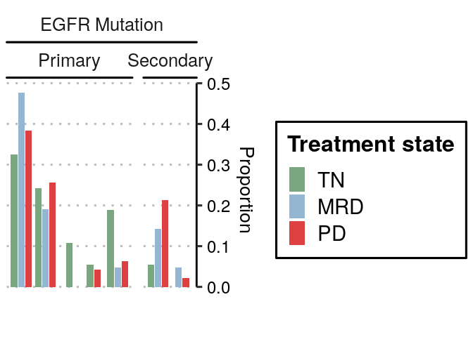
# Instead do as proportion of the timepoints
df_egfr_cat_prop <- egfr_hits %>%
  add_count(facet_group, type_name, name = "n_type") %>%
  complete(facet_group, type_name, fill = list(n_type = 0)) %>%
  add_count(facet_group, name = "n_tp") %>%
  mutate(prop = n_type / n_tp) %>%
  distinct(facet_group, type_name, facet_group, n_type, n_tp, prop, type) %>%
  filter(!is.na(type))
df_egfr_cat_prop$facet_group <- fct_relevel(df_egfr_cat_prop$facet_group, "TN", "MRD", "PD")


egfr_hit_plot_top <- df_egfr_cat_prop %>%
  ggplot(aes(x = (fct_relevel(type_name, var_order)))) +
  geom_col(aes(fill = facet_group, y = prop), position = position_dodge2(preserve = "single")) +
  scale_x_discrete(breaks = var_order, labels = gsub("Primary_|Secondary_", "", var_order)) +
  scale_y_continuous(position = "right") +
  facet_nested(. ~ "EGFR Mutation" + type, space = "free", scales = "free", switch = "y", strip = strip_nested(clip = "off")) +
  scale_fill_manual(values = colors$time_point) +
  guides(
    fill = guide_legend(keywidth = 0.7, keyheight = 1, position = "right"),
    x = guide_axis(cap = "both", angle = 55),
    y = guide_axis(cap = "both")
  ) +
  theme_clean() +
  theme(plot.background = element_blank(), axis.line.y.right = element_line(), strip.placement = "outside", strip.background.x = element_part_rect(linetype = "solid", side = "b", color = "black", fill = NA)) +
  labs(y = "Proportion", x = NULL, fill = "Treatment state")

egfr_hit_plot_top
```
## Combined Plot
```{r, fig.width = 9, fig.height = 16}
spc <- margin(t = 0.2, r = 0.2, b = 0.2, l = 0.2, unit = "lines")

pcomb <- plot_grid(
  swimmers_plot + theme(plot.margin = spc) + coord_cartesian(clip = "off"),
  meta_plot + theme(
    legend.position = "none",
    plot.margin = spc,
    axis.text.y.right = element_blank(),
    axis.ticks.y.right = element_blank(),
    axis.text.x.bottom = element_text(angle = 55),
    strip.clip = "off"
  ) + coord_cartesian(clip = "off"),
  align = "hv",
  nrow = 1, ncol = 2,
  rel_widths = c(1, 0.45),
  axis = "tb"
)

pcomb
```
```{r, fig.width = 12, fig.height = 15.3}
spc <- margin(t = 0.2, r = 0.2, b = 0.2, l = 0.2, unit = "lines")
empty_panel <- plot_spacer() + theme(plot.margin = spc)
pcomb_ext <- plot_grid(
  plotlist = list(
    swimmers_plot + theme(plot.margin = spc) + coord_cartesian(clip = "off"),
    (meta_plot + theme(
      legend.position = "none",
      plot.margin = spc,
      axis.text.y.right = element_blank(),
      axis.ticks.y.right = element_blank(),
      axis.text.x.bottom = element_text(angle = 55),
      strip.clip = "off"
    ) + coord_cartesian(clip = "off")),
    egfr_hit_plot + theme(
      plot.margin = spc, axis.ticks = element_line(color = "black"),
      strip.background.y.right = element_blank(),
      strip.text.y.right = element_blank(),
      axis.title.y.right = element_blank(),
      axis.text.x.bottom = element_text(angle = 55)
    ) + coord_cartesian(clip = "off")
  ),
  align = "hv",
  nrow = 1,
  ncol = 3,
  rel_widths = c(1, 0.4, 0.3),
  axis = "tb"
)
pcomb_ext
ggsave(pcomb_ext, file = here("plots", "swimmers_plus_annos_muts.pdf"), width = 12, height = 15.3)
```
Top Proportion
```{r, fig.width = 3.5, fig.height = 2.5}
egfr_hit_plot_top_final <- egfr_hit_plot_top +
  theme(axis.text.x = element_blank(), axis.ticks.x = element_blank(), axis.line.x = element_blank(), strip.clip = "off", plot.margin = margin(t = 0.25, b = 1.5, l = 0.25, r = 0.25, unit = "lines"), strip.background = element_blank()) +
  coord_cartesian(clip = "off") +
  guides(x = guide_axis(angle = 35, cap = "both"))
egfr_hit_plot_top_final
ggsave(egfr_hit_plot_top_final, file = here("plots", "swimmers_mut_prop_top.pdf"), width = 3.5, height = 2.5)
```
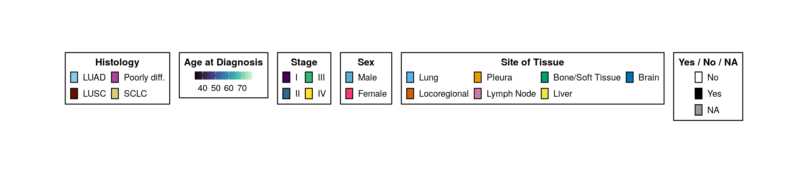
## Legend
```{r, fig.width = 14, fig.height = 3}
lgds <- ggpubr::get_legend(meta_plot)
lgd <- ggpubr::as_ggplot(lgds)
ggsave(lgd, file = here("plots", "swimmers_anno_legend.pdf"), width = 14, height = 3)
lgd
```