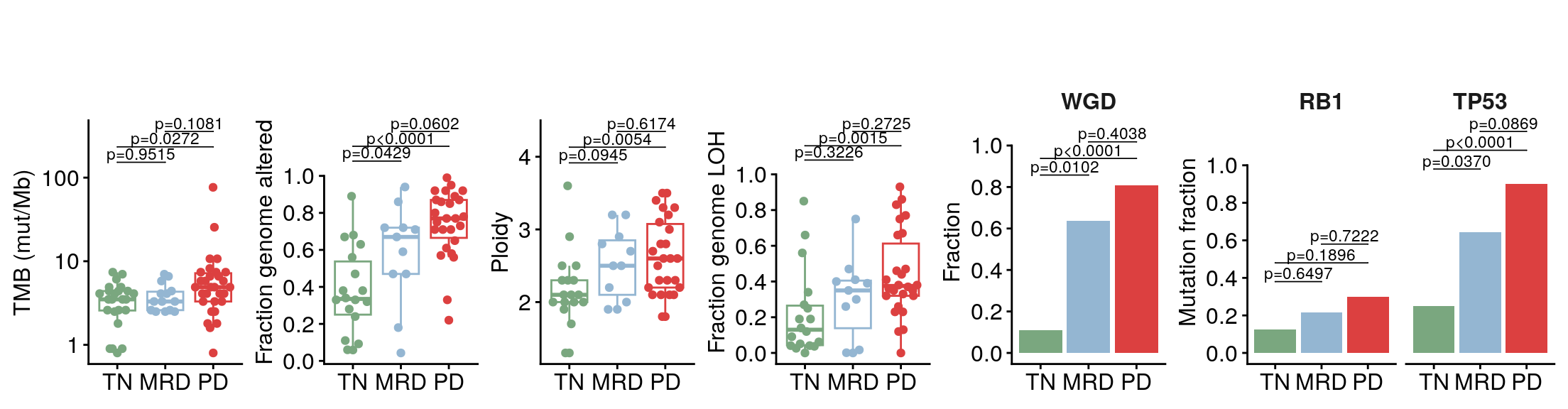
MSK-IMPACT mutation profiles – Figure S2
Genomic characterization of the cohort from the MSK-IMPACT targeted panel: the cohort oncoprint, and the per-timepoint summaries of mutation burden, copy number and TP53/RB1 alteration frequency.
Both panels run off the deposited supplemental workbook. Table S1 supplies the specimen metadata – timepoint, age, TMB, and the FACETS purity/ploidy/FGA/LOH/WGD columns. Table S2 is the de-identified mutation table written by 30_load_impact.qmd: 731 alterations across 292 genes in 68 specimens.
| panel | output |
|---|---|
| S2A |
plots/oncoprint.pdf – cohort oncoprint, 48 genes |
| S2B–G |
plots/impact_genomic_summary.pdf – one composite of six panels: TMB (B), FGA (C), ploidy (D), LOH fraction (E), WGD fraction (F), TP53/RB1 mutation fraction (G) |
Denominators differ across the composite: 68 specimens have MSK-IMPACT (24 TN, 14 MRD, 30 PD) and carry TMB and a mutation profile, of which 55 have an evaluable FACETS fit (18 TN, 11 MRD, 26 PD) and carry FGA, ploidy, LOH and WGD.
Setup
Load data
Code
supp_xlsx <- here("paper_data", "supplemental_tables.xlsx")

# Matched on the table number rather than the full sheet name. S2 was "Table S2 - IMPACT
# Mutations" when this notebook was written and is "Table S2 - IMPACT Muts (snRNA)" in the
# revised workbook; read_excel's error for a missing sheet is clear, but every object below
# then comes up "not found", which reads like a dozen unrelated failures.
supp_sheet <- function(n) {
  sheets <- readxl::excel_sheets(supp_xlsx)
  hit <- grep(sprintf("^Table S%d\\b", n), sheets, value = TRUE)
  if (length(hit) != 1L) {
    stop(sprintf("expected exactly one 'Table S%d' sheet, found: %s",
                 n, paste(hit, collapse = ", ")))
  }
  hit
}

onco_dat <- readxl::read_excel(supp_xlsx, sheet = supp_sheet(2))

metadata <- readxl::read_excel(supp_xlsx, sheet = supp_sheet(1)) %>%
  as.data.frame()

# The workbook stores these as text so that "NA" survives the round trip.
for (v in c("facets_purity", "facets_ploidy", "facets_fga", "facets_frac_loh")) {
  metadata[[v]] <- suppressWarnings(as.numeric(metadata[[v]]))
}
metadata$facets_wgd <- as.logical(metadata$facets_wgd)
metadata$time_point <- fct_relevel(metadata$time_point, "TN", "MRD", "PD")

# TMB comes straight off Table S1, which is keyed on sample_id. The internal route reads it
# from the IMPACT clinical table (CVR_TMB_SCORE), reached through the DMP sample barcode;
# neither the barcode nor the clinical table travels with the deposit. Table S1 records the
# same value under impact_tmb, for the 68 specimens with a panel result.
metadata$tmb <- suppressWarnings(as.numeric(metadata$impact_tmb))
stopifnot(sum(!is.na(metadata$tmb)) == 68L)

rownames(metadata) <- metadata$sample_id
Figure S2A – cohort oncoprint
One column per specimen, one row per gene, cells collapsed to a simplified mutation type. Specimens with no alteration at all would drop out of the pivot; none exist here, so the 68 columns are the 68 IMPACT specimens.
Code
comut_mat_final <- onco_dat %>%
  pivot_wider(
    id_cols = sample_id, names_from = gene, values_from = mutation_type_simple,
    values_fn = function(x) paste0(x, collapse = ";"), values_fill = ""
  ) %>%
  column_to_rownames("sample_id") %>%
  as.matrix() %>%
  t()

# Everything downstream indexes the metadata by the matrix columns, so the two stay aligned
# and the boxplot denominators are the IMPACT specimens rather than the full cohort.
impact_meta <- metadata[colnames(comut_mat_final), ]
stopifnot(!anyNA(impact_meta$sample_id))

tp_counts <- paste(names(table(impact_meta$time_point)), table(impact_meta$time_point))
cli::cli_alert_info("{ncol(comut_mat_final)} specimen{?s} with MSK-IMPACT: {tp_counts}.")

mut_pal <- c(
  "Missense Mutation" = "#1C91D4",
  "Nonsense Mutation" = "#D5C711",
  "Deep Deletion" = "blue",
  "Amplification" = "red",
  "Frameshift Indel" = "#D55E00",
  "Inframe Indel" = "#CC79A7",
  "RNA Fusion" = "#F0E442",
  "Structural Variant" = "#56B4E9",
  "Other" = "#007756"
)

stopifnot(all(onco_dat$mutation_type_simple %in% names(mut_pal)))
Copy number and fusion events fill the cell; point mutations and indels are drawn as a centred band so a gene carrying both stays readable.
Code
alter_fun <- list(
  background = alter_graphic("rect", fill = "#CCCCCC"),
  "Amplification" = alter_graphic("rect", fill = mut_pal["Amplification"]),
  "Deep Deletion" = alter_graphic("rect", fill = mut_pal["Deep Deletion"]),
  "Missense Mutation" = alter_graphic("rect", height = 0.33, fill = mut_pal["Missense Mutation"]),
  "Nonsense Mutation" = alter_graphic("rect", height = 0.33, fill = mut_pal["Nonsense Mutation"]),
  "Frameshift Indel" = alter_graphic("rect", height = 0.33, fill = mut_pal["Frameshift Indel"]),
  "Inframe Indel" = alter_graphic("rect", height = 0.33, fill = mut_pal["Inframe Indel"]),
  "RNA Fusion" = alter_graphic("rect", height = 1, width = 0.33, fill = mut_pal["RNA Fusion"]),
  "Structural Variant" = alter_graphic("rect", height = 0.33, fill = mut_pal["Structural Variant"]),
  "Other" = alter_graphic("rect", height = 0.33, fill = mut_pal["Other"])
)

anno_cols <- list(
  "timepoint" = colors$time_point,
  "WGD" = c("TRUE" = "black", "FALSE" = "white", "NA" = "grey80"),
  "FGA" = circlize::colorRamp2(
    seq(min(impact_meta$facets_fga, na.rm = TRUE), max(impact_meta$facets_fga, na.rm = TRUE), length.out = 10),
    viridis::mako(10)
  ),
  "age" = circlize::colorRamp2(
    seq(min(impact_meta$age_at_intial_diagnosis, na.rm = TRUE), max(impact_meta$age_at_intial_diagnosis, na.rm = TRUE), length.out = 10),
    viridis::mako(10)
  )
)

tmb_breaks <- c(1, 10, 100)

top_anno <- HeatmapAnnotation(
  na_col = "white",
  annotation_name_side = "left",
  annotation_label = c("TMB", "FGA", "WGD", "Age", "Time point"),
  # Bar heights are log10(TMB + 1) so that a TMB of 0 still lands on the axis; the ticks
  # are placed at the same shift and labelled on the original scale.
  TMB = anno_barplot(
    x = log10(impact_meta$tmb + 1),
    axis_param = list(
      at = log10(tmb_breaks + 1),
      labels = tmb_breaks,
      side = "left"
    ),
    ylim = c(log10(1), log10(100)),
    border = FALSE,
    baseline = 0
  ),
  FGA = anno_simple(impact_meta$facets_fga, col = anno_cols$FGA, na_col = "grey80"),
  WGD = anno_simple(as.character(impact_meta$facets_wgd), col = c("TRUE" = "black", "FALSE" = "white"), na_col = "grey80"),
  age = impact_meta$age_at_intial_diagnosis,
  timepoint = anno_block(
    gp = gpar(fill = colors$time_point),
    labels = c("Treatment Naive", "MRD", "Progressive Disease"),
    labels_gp = gpar(col = "white", fontsize = 11)
  ),
  col = anno_cols
)
Genes altered in at least 10% of specimens, unioned with a curated panel of canonical MAPK/RTK, PI3K and cell-cycle genes. The frequency rule alone returns 10 genes and drops the recurrent-but-rare targetable events the figure is there to show. The curated list was frozen from the OncoKB-annotated genes altered in the cohort.
Code
min_mut_freq <- 0.1

mut_freq <- (apply(comut_mat_final, MARGIN = 1, function(x) sum(x != "")) / ncol(comut_mat_final)) %>%
  sort(decreasing = TRUE)

plot_genes <- names(which(mut_freq >= min_mut_freq))

add_genes <- c(
  "KRAS", "BRAF", "MAPK1", "MAP2K4", "MAP3K1", "NF1", "SPRED1",
  "LZTR1", "PTPN11", "GAB2", "IRS2", "RAC1", "PAK1", "ERBB2", "ALK",
  "MET", "RET", "ROS1", "KIT", "PDGFRA", "FGFR1", "KDR", "NTRK1",
  "EPHA3", "EML4", "JUN", "ETV1", "PIK3CA", "PIK3R1", "AKT1", "AKT2",
  "MTOR", "RICTOR", "INPP4B", "YAP1", "CDK4", "CCND1", "CCNE1"
)

# A curated gene with no alteration in the cohort is not a matrix row, and would subset to
# NA rather than error.
stopifnot(all(add_genes %in% rownames(comut_mat_final)))

plot_genes <- unique(c(plot_genes, add_genes))

# The published panel is 48 genes carrying 309 of the 731 alterations; assert both, so a
# change in Table S2 or in the curated list surfaces here and not in the PDF.
stopifnot(length(plot_genes) == 48L)
stopifnot(sum(onco_dat$gene %in% plot_genes) == 309L)
Code
gene_frac <- rowMeans(comut_mat_final[plot_genes, ] != "")

ht <- oncoPrint(comut_mat_final[plot_genes, ],
  right_annotation = rowAnnotation(
    Proportion = anno_barplot(gene_frac,
      border = FALSE, width = unit(3, "cm"),
      axis_param = list(
        at = c(0, 0.5, 1), labels = c("0", "0.5", "1"),
        labels_rot = 0, side = "top"
      ),
      outline = FALSE
    ),
    annotation_name_side = "top"
  ),
  top_annotation = top_anno,
  column_split = impact_meta$time_point,
  column_title = NULL,
  alter_fun = alter_fun,
  col = mut_pal,
  show_column_names = TRUE,
  remove_empty_columns = FALSE,
  column_title_rot = 0,
  border = TRUE
)

# FGA and WGD are drawn with anno_simple, which carries no legend of its own; Age is a plain
# vector annotation and brings one. merge_legend collects all of them into a single column.
lgd_fga <- Legend(col_fun = anno_cols$FGA, title = "FGA")
lgd_wgd <- Legend(
  labels = c("TRUE", "FALSE", "NA"),
  legend_gp = gpar(fill = c("TRUE" = "black", "FALSE" = "white", "NA" = "grey80")),
  title = "WGD"
)

draw_oncoprint <- function() {
  suppressWarnings(draw(ht,
    annotation_legend_list = list(lgd_fga, lgd_wgd),
    merge_legend = TRUE,
    heatmap_legend_side = "right",
    annotation_legend_side = "right",
    show_annotation_legend = FALSE
  ))
  # anno_barplot draws no axis line on a right annotation; add the two the panel needs.
  decorate_annotation("Proportion", {
    grid.lines(x = unit(c(0, 0), "npc"), y = unit(c(0, 1), "npc"), gp = gpar(lwd = 1))
    grid.lines(x = unit(c(0, 1), "npc"), y = unit(c(1, 1), "npc"), gp = gpar(lwd = 1))
  })
}

pdf(file = here("plots", "oncoprint.pdf"), width = 14, height = 11)
draw_oncoprint()
dev.off()
png
2 Code
draw_oncoprint()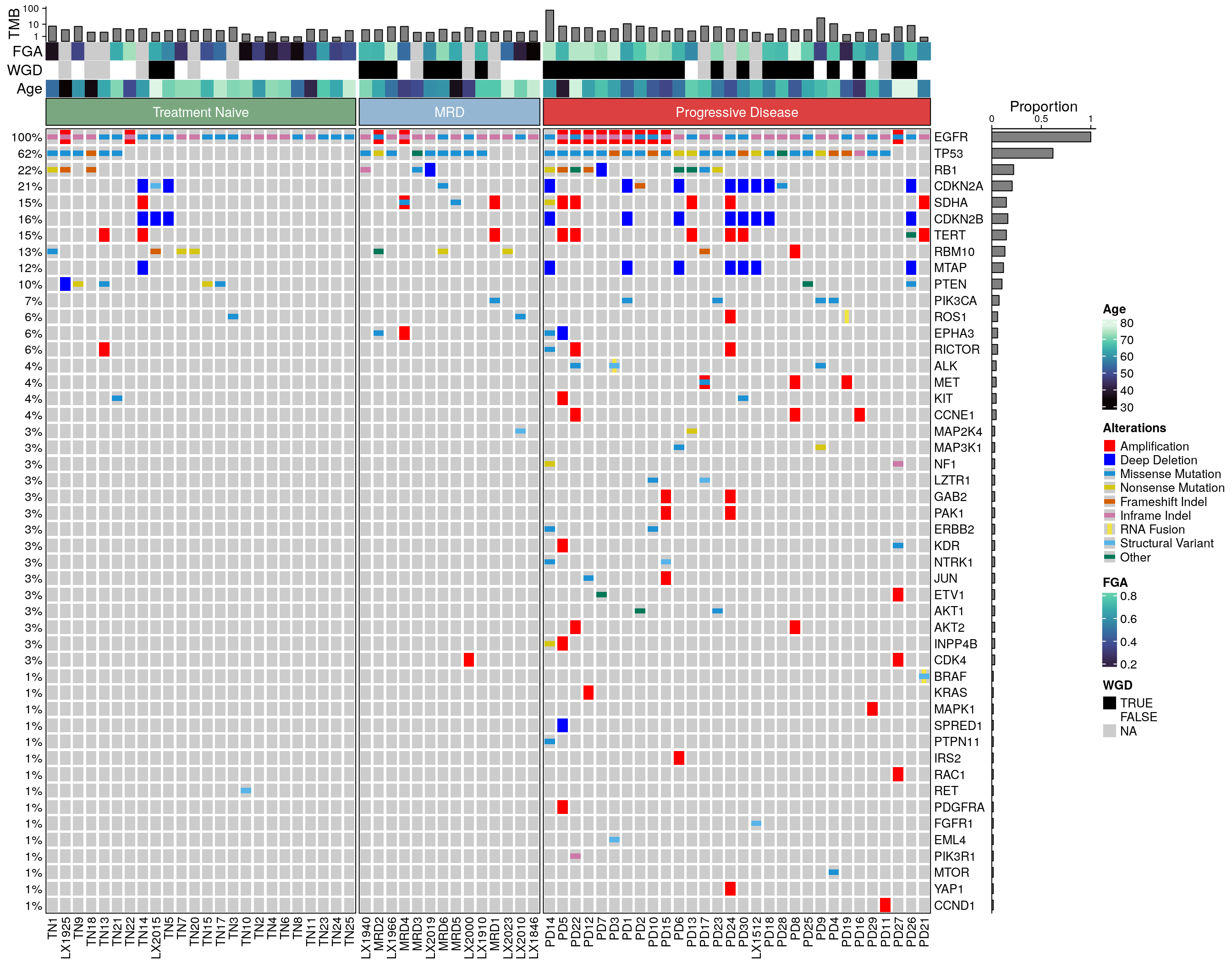
Figure S2B–G – genomic summaries
Six panels saved as one composite. B–E are two-sided Wilcoxon rank-sum tests, F and G pairwise two-sided Fisher’s exact tests; all print the exact p value and none are corrected for multiple testing, matching the legend.
Code
my_comparisons <- list(c("TN", "MRD"), c("TN", "PD"), c("MRD", "PD"))

format_pval <- scales::label_pvalue(accuracy = 0.0001, add_p = TRUE)

# y_range: c(min, max) of the axis in plot space (log10 values for a log-scaled axis). The
# brackets sit at fixed proportions of that range, so the three stack the same way whatever
# the units of the panel.
compute_wilcox_stats <- function(df, var, y_range, frac_start = 0.08, frac_step = 0.08) {
  range_size <- diff(y_range)
  map(my_comparisons, function(comp) {
    d1 <- df[[var]][df$time_point == comp[1]]
    d2 <- df[[var]][df$time_point == comp[2]]
    tibble(group1 = comp[1], group2 = comp[2], p.value = wilcox.test(d1, d2)$p.value)
  }) %>%
    list_rbind() %>%
    mutate(
      y.position = y_range[2] + range_size * seq(frac_start, by = frac_step, length.out = n()),
      label = format_pval(p.value)
    )
}
Code
# TMB: tested and plotted on log10, so the brackets sit at even spacing on the drawn axis.
tmb_df <- impact_meta %>%
  filter(!is.na(tmb)) %>%
  mutate(log_tmb = log10(tmb))
tmb_stats <- compute_wilcox_stats(tmb_df, "log_tmb", y_range = c(log10(0.5), log10(100)))

p1 <- tmb_df %>%
  ggplot(aes(x = time_point, y = log_tmb)) +
  ggbeeswarm::geom_quasirandom(aes(color = time_point)) +
  geom_boxplot(fill = NA, outlier.shape = NA, aes(color = time_point)) +
  scale_y_continuous(breaks = log10(c(1, 10, 100)), labels = c(1, 10, 100)) +
  theme_classic() +
  ggpubr::stat_pvalue_manual(tmb_stats, label = "label", tip.length = 0, size = 3) +
  labs(x = "Timepoint", y = "TMB (mut/Mb)") +
  scale_color_manual(values = colors$time_point) +
  coord_cartesian(clip = "off") +
  theme(legend.position = "none", plot.margin = margin(t = 2, unit = "lines"))

fga_stats <- compute_wilcox_stats(impact_meta %>% filter(!is.na(facets_fga)), "facets_fga", y_range = c(0, 1))

p2 <- impact_meta %>%
  filter(!is.na(facets_fga)) %>%
  ggplot(aes(x = time_point, y = facets_fga)) +
  ggbeeswarm::geom_quasirandom(aes(color = time_point)) +
  geom_boxplot(fill = NA, outlier.shape = NA, aes(color = time_point)) +
  theme_classic() +
  ggpubr::stat_pvalue_manual(fga_stats, label = "label", tip.length = 0, size = 3) +
  labs(x = "Timepoint", y = "Fraction genome altered") +
  scale_y_continuous(breaks = seq(0, 1, by = 0.2)) +
  scale_color_manual(values = colors$time_point) +
  guides(y = guide_axis(cap = "upper")) +
  coord_cartesian(clip = "off") +
  theme(legend.position = "none", plot.margin = margin(t = 2, unit = "lines"))

ploidy_stats <- compute_wilcox_stats(impact_meta %>% filter(!is.na(facets_ploidy)), "facets_ploidy", y_range = c(1, 3.7))

p3 <- impact_meta %>%
  filter(!is.na(facets_ploidy)) %>%
  ggplot(aes(x = time_point, y = facets_ploidy)) +
  ggbeeswarm::geom_quasirandom(aes(color = time_point)) +
  geom_boxplot(fill = NA, outlier.shape = NA, aes(color = time_point)) +
  theme_classic() +
  ggpubr::stat_pvalue_manual(ploidy_stats, label = "label", tip.length = 0, size = 3) +
  labs(x = "Timepoint", y = "Ploidy") +
  scale_color_manual(values = colors$time_point) +
  coord_cartesian(clip = "off") +
  theme(legend.position = "none", plot.margin = margin(t = 2, unit = "lines"))

loh_stats <- compute_wilcox_stats(impact_meta %>% filter(!is.na(facets_frac_loh)), "facets_frac_loh", y_range = c(0, 1))

p4 <- impact_meta %>%
  filter(!is.na(facets_frac_loh)) %>%
  ggplot(aes(x = time_point, y = facets_frac_loh)) +
  ggbeeswarm::geom_quasirandom(aes(color = time_point)) +
  geom_boxplot(fill = NA, outlier.shape = NA, aes(color = time_point)) +
  theme_classic() +
  ggpubr::stat_pvalue_manual(loh_stats, label = "label", tip.length = 0, size = 3) +
  labs(x = "Timepoint", y = "Fraction genome LOH") +
  scale_y_continuous(breaks = seq(0, 1, by = 0.2)) +
  scale_color_manual(values = colors$time_point) +
  guides(y = guide_axis(cap = "upper")) +
  coord_cartesian(clip = "off") +
  theme(legend.position = "none", plot.margin = margin(t = 2, unit = "lines"))
WGD is a proportion rather than a distribution, so the brackets are Fisher’s exact tests on the 2x2 of WGD status by timepoint, over the 55 specimens with an evaluable FACETS fit.
Code
wgd_counts <- impact_meta %>%
  dplyr::filter(!is.na(facets_wgd)) %>%
  dplyr::count(time_point, facets_wgd) %>%
  tidyr::complete(time_point, facets_wgd, fill = list(n = 0L)) %>%
  group_by(time_point) %>%
  mutate(nn = sum(n), wgd_frac = n / nn) %>%
  ungroup()

wgd_fisher <- map(my_comparisons, .f = function(comp) {
  mat <- wgd_counts %>%
    filter(time_point %in% comp) %>%
    select(time_point, facets_wgd, n) %>%
    pivot_wider(names_from = facets_wgd, values_from = n, values_fill = 0L) %>%
    column_to_rownames("time_point") %>%
    as.matrix()
  # fisher.test is orientation-agnostic for the p value, but fixing the order keeps the
  # odds ratio reported in the tidied result the right way up.
  stats::fisher.test(mat[comp, c("TRUE", "FALSE"), drop = FALSE]) %>%
    broom::tidy() %>%
    mutate(group1 = comp[1], group2 = comp[2])
}) %>%
  list_rbind() %>%
  mutate(
    y.position = seq(max(wgd_counts$wgd_frac[wgd_counts$facets_wgd == TRUE]) + 0.05,
      by = 0.08, length.out = n()
    ),
    label = format_pval(p.value)
  )

# The single bar is facetted so it carries a strip label matching the two-gene panel beside it.
p5 <- wgd_counts %>%
  filter(facets_wgd == TRUE) %>%
  mutate(.facet = "WGD") %>%
  ggplot(aes(x = time_point, y = wgd_frac)) +
  geom_col(aes(fill = time_point)) +
  facet_wrap(~.facet) +
  labs(y = "Fraction") +
  scale_y_continuous(breaks = seq(0, 1, by = 0.2)) +
  scale_fill_manual(values = colors$time_point) +
  guides(y = guide_axis(cap = "upper")) +
  theme_classic() +
  ggpubr::stat_pvalue_manual(wgd_fisher, label = "label", tip.length = 0, size = 3) +
  coord_cartesian(clip = "off", ylim = c(0, max(wgd_fisher$y.position) + 0.05)) +
  theme(
    legend.position = "none",
    strip.background = element_blank(),
    strip.text = element_text(face = "bold", size = 12)
  )
TP53 and RB1 alteration frequency, over all 68 specimens with a panel result. Any alteration type counts, so the denominator is the oncoprint column count and not the FACETS subset.
Code
test_genes <- c("TP53", "RB1")

mut_by_tp <- (comut_mat_final != "") %>%
  as.data.frame() %>%
  rownames_to_column(var = "Gene") %>%
  tidyr::pivot_longer(cols = !Gene, names_to = "sample_id") %>%
  dplyr::left_join(impact_meta[, c("sample_id", "time_point")], by = "sample_id") %>%
  dplyr::group_by(Gene, time_point) %>%
  dplyr::summarise(n_mut = sum(value), n_total = n(), .groups = "drop") %>%
  dplyr::mutate(frac_mut = n_mut / n_total)

enrich_res <- map(test_genes, .f = function(gene) {
  map(my_comparisons, .f = function(comp) {
    d <- mut_by_tp %>% filter(Gene == gene, time_point %in% comp)
    mat <- matrix(c(d$n_mut, d$n_total - d$n_mut),
      nrow = 2, byrow = FALSE,
      dimnames = list(d$time_point, c("Mut", "Wt"))
    )
    stats::fisher.test(mat) %>%
      broom::tidy() %>%
      mutate(Gene = gene, group1 = comp[1], group2 = comp[2])
  }) %>% list_rbind()
}) %>%
  list_rbind() %>%
  group_by(Gene) %>%
  mutate(
    y.position = seq(
      from = max(mut_by_tp$frac_mut[mut_by_tp$Gene == dplyr::first(Gene)]) + 0.08,
      by = 0.1,
      length.out = n()
    ),
    label = format_pval(p.value)
  ) %>%
  ungroup()

p6 <- mut_by_tp %>%
  filter(Gene %in% test_genes) %>%
  mutate(Gene = factor(Gene, levels = test_genes)) %>%
  # fill stays inside geom_col: on the global aes the bracket layer inherits it, and the
  # bracket data has no time_point column.
  ggplot(aes(x = time_point, y = frac_mut)) +
  geom_col(aes(fill = time_point)) +
  facet_wrap(~Gene, nrow = 1) +
  scale_fill_manual(values = colors$time_point) +
  ggpubr::stat_pvalue_manual(enrich_res, label = "label", tip.length = 0, size = 3) +
  labs(y = "Mutation fraction", x = NULL, fill = "Timepoint") +
  scale_y_continuous(breaks = seq(0, 1, by = 0.2)) +
  theme_classic() +
  coord_cartesian(clip = "off") +
  guides(y = guide_axis(cap = "upper")) +
  theme(
    legend.position = "none",
    strip.background = element_blank(),
    strip.text = element_text(face = "bold", size = 12)
  )
Code
pcomb <- (p1 | p2 | p3 | p4 | p5 | p6) +
  plot_layout(guides = "collect", widths = c(1, 1, 1, 1, 1, 2)) &
  guides(x = guide_axis(angle = 0)) & labs(x = NULL) &
  theme(
    plot.margin = margin(t = 1.5, 0.25, 0.25, 0.25, unit = "lines"),
    axis.text = element_text(size = 12),
    axis.title = element_text(size = 12),
    legend.text = element_text(size = 12),
    legend.title = element_text(size = 15)
  )

ggsave(pcomb, filename = here("plots", "impact_genomic_summary.pdf"), width = 11.5, height = 3)

pcomb