---
title: "Figure 3 and S6-S8 -- LUAD deprogramming towards stem-like states"
author: "Matthew Zatzman"
execute:
warning: false
error: false
format:
html:
code-fold: true
code-tools: true
toc: true
---
Figure 3 and the supplementary figures its legend points to: S6 (epithelial cell
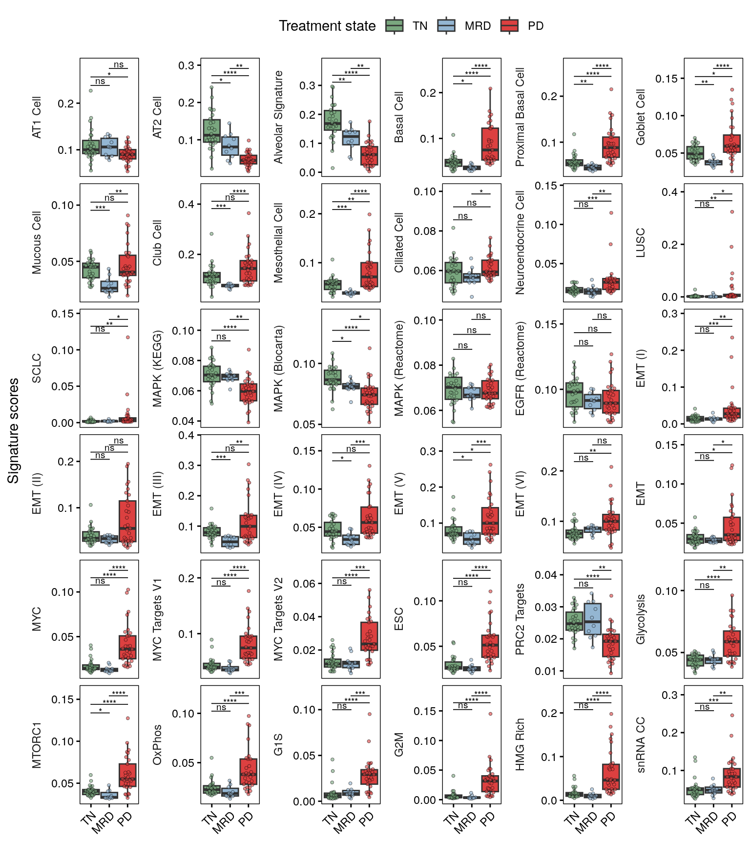
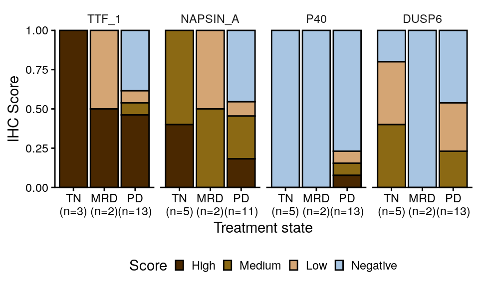
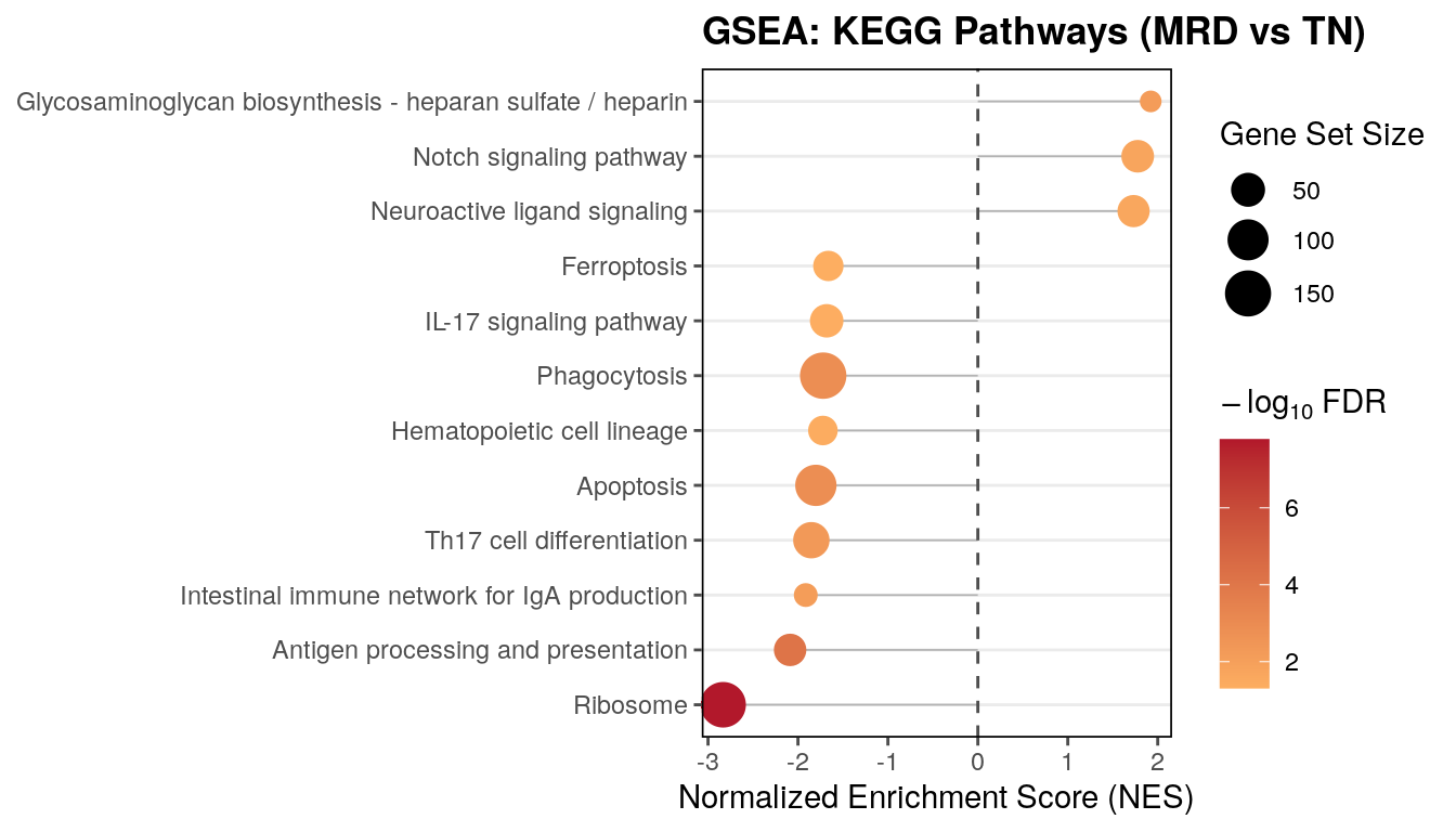
state annotation), S7 (tumor cell signatures and IHC) and S8 (gene-set enrichment
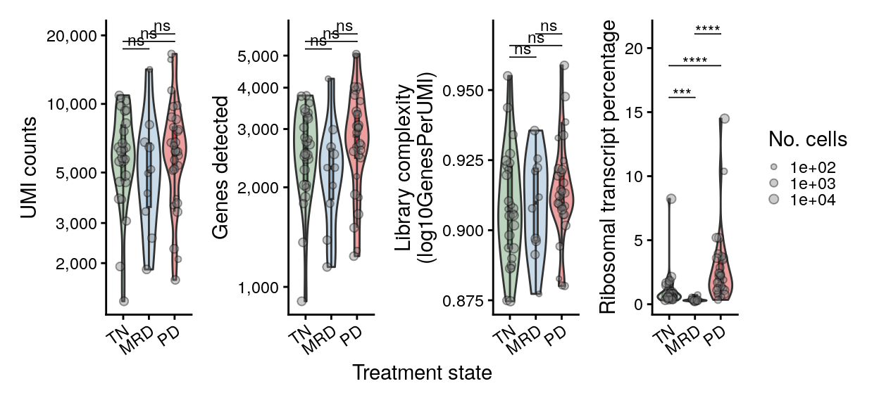
and tumor-cell library quality).
S7A reuses the signature summary built for Figure 3C/3G, so those chunks stay
together in this document.
Run `00_download_convert.qmd` first to build `paper_data/`.
{{< include _setup.qmd >}}
# Load data
The cohort, epithelial and tumor objects. `tum` is derived from `epi`, so asking
for it implies reading `epi`. No inferCNV or histotime object is needed.
```{r load}
# L'Ecuyer-CMRG so forked mclapply workers get reproducible streams.
RNGkind("L'Ecuyer-CMRG")
set.seed(42)

db <- load_project(objects = c("cohort", "epi", "tum"))

srt     <- db$srt
srt_epi <- db$srt_epi
srt_tum <- db$srt_tum
```
## Cohort metadata, pathways and IHC
`metadata` is Table S1 as published: one row per reported specimen, 73 rows. The
two-core MRD2 merge is already applied both here and in the objects, so nothing in
this notebook needs to reconcile libraries against specimens.
```{r metadata}
metadata <- readxl::read_excel(here("paper_data", "supplemental_tables.xlsx"),
                               sheet = "Table S1 - Cohort Metadata") %>%
  as.data.frame()
for (v in c("facets_fga", "facets_ploidy", "facets_purity", "facets_frac_loh")) {
  metadata[[v]] <- as.numeric(metadata[[v]])
}
metadata$facets_wgd <- as.logical(metadata$facets_wgd)
metadata$time_point <- fct_relevel(metadata$time_point, "TN", "MRD", "PD")
metadata$sample_id  <- fct_relevel(metadata$sample_id, names(colors$sample_id))
stopifnot(nrow(metadata) == 73, !any(duplicated(metadata$sample_id)))

# Sample-level view used by the composition and cellularity panels.
meta_final <- metadata
meta_final$sample_has_tumor <- meta_final$sample_id %in% unique(srt_tum$sample_id)
```
```{r pathways}
pathways <- read.table(here("paper_data", "egfr_pathways_annotations.txt"),
                       header = TRUE, sep = "\t")
mapk_paths <- filter(pathways, category == "MAPK")$pathway
tum_paths  <- c("LUAD", "LUSC", "SCLC")

# The signature columns on the objects use the short names; the pathway tables use the
# source names. Rename the tables, not the objects.
rename_sigs <- function(df) {
  df$pathway[df$pathway == "LUAD_GIRARD"] <- "LUAD"
  df$pathway[df$pathway == "LUSC_GIRARD"] <- "LUSC"
  df$pathway[df$pathway == "SCLC_CCLE"]   <- "SCLC"
  df
}
pathways <- rename_sigs(pathways)

# Named separately because S9A/S9E use its gene lists directly. Deliberately not passed
# through rename_sigs() -- the v2 names are what the GSEA TERM2GENE mapping expects.
pathways_v2 <- read.table(here("paper_data", "egfr_pathways_v2.txt"),
                          header = TRUE, sep = "\t")
pathways_v2_t2g <- pathways_v2 %>% dplyr::relocate(pathway, Gene)

# pathways_full adds the v2 set and the 67 Tirosh metaprograms, which together define the
# `mp*` score columns carried on srt_epi / srt_tum.
pathways_full <- bind_rows(
  pathways_v2,
  read.csv(here("paper_data", "tirosh_mps_67_natcan_2025.csv")) %>%
    dplyr::rename(pathway = Geneset) %>%
    dplyr::select(pathway, Gene)
) %>% rename_sigs()
```
The IHC table is keyed on `sample_id`, so it joins to `meta_final` directly. It covers 24
of the 73 specimens; the rest were not stained.
```{r ihc}
ihc <- readr::read_csv(here("paper_data", "nucseq_ihc_public.csv"),
                       show_col_types = FALSE) %>%
  # The source column is misspelled "cytoplsmic". Without this rename it fails
  # ends_with("_cytoplasmic") below and is silently left out of the pivot, and since the
  # S7B panel then drops DUSP6 Nuclear as well, DUSP6 disappears from `gene` entirely and
  # fct_relevel(gene, sel_stains) errors on the absent level. Upstream renames it too.
  dplyr::rename("dusp6_cytoplasmic" = "dusp6_cytoplsmic") %>%
  inner_join(meta_final, by = "sample_id") %>%
  dplyr::relocate(sample_id, time_point, scrna_histology, .before = 1)

ihc_long <- ihc %>%
  pivot_longer(cols = c(ends_with("_cytoplasmic"), ends_with("_nuclear")),
               values_to = "value", names_to = "stain") %>%
  mutate(value = as.numeric(value)) %>%
  mutate(
    gene = str_to_upper(gsub("_cytoplasmic|_nuclear", "", stain)),
    stain_loc = ifelse(grepl("cytoplasmic", stain), "Cytoplasmic", "Nuclear"),
    time_point = fct_relevel(time_point, "TN", "MRD")
  ) %>%
  filter(!is.na(value), !is.na(time_point)) %>%
  group_by(stain) %>%
  mutate(value_z = scale(value)[, 1]) %>%
  ungroup() %>%
  mutate(gene_lab = ifelse(stain_loc == "Cytoplasmic", glue("{gene} (C)"), glue("{gene} (N)"))) %>%
  mutate(osi_exp = ifelse(time_point %in% c("MRD", "PD"), "Exp", "TN")) %>%
  filter(sample_id %in% srt_tum$sample_id) %>%
  mutate(score_cat = case_when(
    value < 10 ~ "Negative",
    value >= 10 & value < 100 ~ "Low",
    value >= 100 & value < 200 ~ "Medium",
    value >= 200 ~ "High"
  )) %>%
  mutate(score_cat = factor(score_cat, levels = c("Negative", "Low", "Medium", "High")))

meta_final$has_ihc <- meta_final$sample_id %in% ihc_long$sample_id
```
# Figure 3 -- LUAD deprogramming towards stem-like states
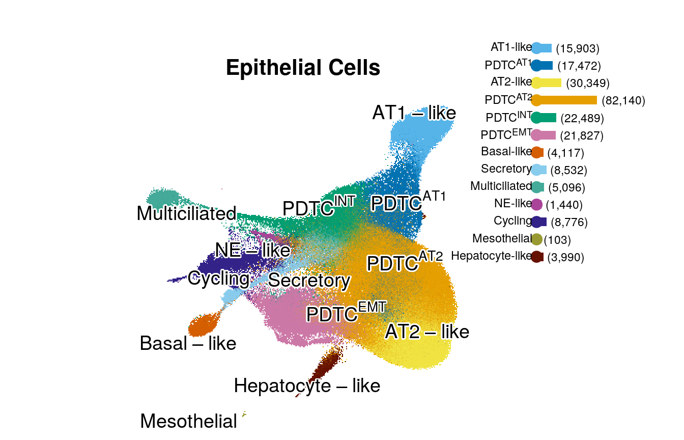
## Figure 3A -- epithelial UMAP by cell type
```{r fig3a-epi-umap, fig.width = 7, fig.height = 4.5}
lab_cents <- scatools:::get_label_centers(obj = srt_epi, group_var = "cell_type_epi", reduced_dim = "umap")

df_leg <- srt_epi@meta.data %>%
  add_count(cell_type_epi, name = "epi_n") %>%
  distinct(cell_type_epi, epi_n) %>%
  mutate(label = glue("({prettyNum(epi_n, big.mark = ',')})"))

p1_leg <- df_leg %>%
  ggplot(aes(y = fct_rev(cell_type_epi), x = epi_n)) +
  geom_point(aes(x = -6000, color = cell_type_epi), size = 3.5) +
  geom_col(aes(fill = cell_type_epi), width = 0.5) +
  geom_text(aes(x = epi_n, label = label), size = 3, hjust = -0.1, color = "black", parse = F) +
  scale_fill_manual(values = colors$cell_type_epi) +
  scale_color_manual(values = colors$cell_type_epi) +
  coord_cartesian(clip = "off") +
  # facet_grid(fct_relevel(cell_type_l2, "Myeloid", "TNK", "B/Plasma", "Stroma", "Other") ~ ., scales = "free", space = "free", switch = "y") +
  scale_y_discrete(labels = label_md) +
  theme(
    strip.placement = "outside",
    strip.background.y = element_part_rect(side = "r", fill = NA),
    axis.ticks = element_blank(),
    axis.line = element_blank(),
    axis.text.x = element_blank(),
    axis.text.y = ggtext::element_markdown(),
    strip.text.y.left = element_text(angle = 0, hjust = 1),
    plot.margin = margin(1, 4, 1, 1, unit = "lines")
  ) +
  labs(x = NULL, y = NULL) +
  scale_x_continuous(expand = c(0.025, 0)) +
  guides(x = guide_axis(cap = "both")) +
  NoLegend()

p1 <- DimPlot(srt_epi, reduction = "umap", group.by = "cell_type_epi", shuffle = T, raster.dpi = c(350, 350)) +
  umap_theme() +
  ggrepel::geom_text_repel(
    data = lab_cents, aes(x = x, y = y, label = label_plotmath(cell_type_epi)),
    parse = TRUE,
    size = 5,
    min.segment.length = Inf,
    segment.size = 1.5,
    fontface = "bold",
    force = 5,
    bg.colour = "white",
    max.iter = 1e9,
    bg.r = 0.1,
    position = ggpp::position_nudge_center(center_x = 0, center_y = 0, direction = "radial", x = 0, y = 0)
  ) +
  scale_color_manual(values = colors$cell_type_epi, labels = label_num_generator(srt_epi$cell_type_epi), breaks = levels(srt_epi$cell_type_epi)) +
  NoAxes() +
  NoLegend() +
  theme(aspect.ratio = 1) +
  labs(title = "Epithelial Cells")

layout <- c(
  area(t = 10, b = 100, l = 1, r = 100),
  area(t = 4, l = 88, b = 59, r = 100)
)
# pcomb <- (p1 + theme(plot.margin = margin())) + free(p1_leg + theme(aspect.ratio = 1.9, plot.margin = margin())) + plot_layout(design = layout)
pcomb <- (p1 + theme(plot.margin = margin())) + p1_leg + plot_layout(design = layout)

ggsave(pcomb, file = here("plots", "epi_umap.pdf"), width = 7, height = 4.5)
pcomb
```
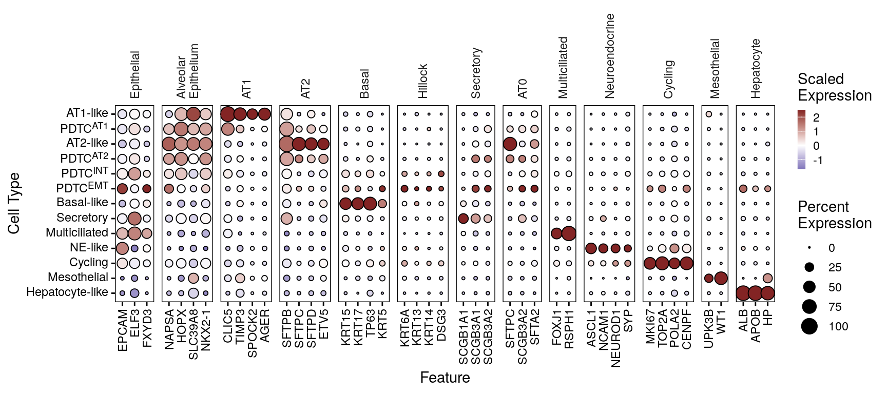
## Figure 3B -- epithelial cell type marker dot plot
```{r fig3b-epi-marker-dotplot, fig.width = 9, fig.height = 4}
# DotPlotter() picks its own scales, so the state labels are markdown-ified on the
# levels rather than through scale_y_discrete().
epi_dotplot <- DotPlotter(md_epi_states(srt_epi[, srt_epi$cell_type_epi != "PD9/PD27 unk."]), features = markers$epi_markers_final, group.by = "cell_type_epi", cluster_groups = F, rotate_y_strip = T) +
  theme(axis.text.y = element_markdown())
epi_dotplot
ggsave(epi_dotplot, file = here("plots", "epi_marker_dotplot.pdf"), width = 9, height = 4)
```
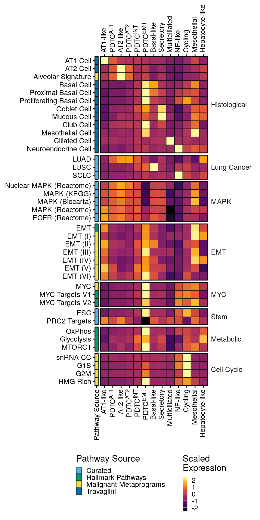
## Figure 3C -- signature heatmap across epithelial cell types
Proportions of non-malignant cells across samples
```{r, fig.width = 8, fig.height = 9}
emt_paths <- grep("emt|HALLMARK_EPITHELIAL_MESENCHYMAL_TRANSITION", ignore.case = T, colnames(srt_epi@meta.data), value = T)
myc_paths <- c(grep("myc", ignore.case = T, colnames(srt_epi@meta.data), value = T))
stemness <- c("WONG_EMBRYONIC_STEM_CELL_CORE", "BENPORATH_PRC2_TARGETS")
metabolic_paths <- c("HALLMARK_GLYCOLYSIS", "HALLMARK_OXIDATIVE_PHOSPHORYLATION", "HALLMARK_MTORC1_SIGNALING")
histological_malignant <- c("LUAD", "LUSC", "SCLC")
histological <- c("TRAVAGLINI_LUNG_ALVEOLAR_EPITHELIAL_TYPE_1_CELL", "TRAVAGLINI_LUNG_ALVEOLAR_EPITHELIAL_TYPE_2_CELL", "mp44_alveolar", "TRAVAGLINI_LUNG_BASAL_CELL", "TRAVAGLINI_LUNG_CILIATED_CELL", "TRAVAGLINI_LUNG_CLUB_CELL", "TRAVAGLINI_LUNG_NEUROENDOCRINE_CELL", "TRAVAGLINI_LUNG_PROLIFERATING_BASAL_CELL", "TRAVAGLINI_LUNG_PROXIMAL_BASAL_CELL", "TRAVAGLINI_LUNG_GOBLET_CELL", "TRAVAGLINI_LUNG_MUCOUS_CELL", "TRAVAGLINI_LUNG_MESOTHELIAL_CELL")
cell_cycle <- c(grep("cycle", colnames(srt_epi@meta.data), ignore.case = T, value = T))
mapk <- c("REACTOME_MAPK_FAMILY_SIGNALING_CASCADES", "REACTOME_MAPK_TARGETS_NUCLEAR_EVENTS_MEDIATED_BY_MAP_KINASES", "BIOCARTA_MAPK_PATHWAY", "KEGG_MAPK_SIGNALING_PATHWAY", "REACTOME_SIGNALING_BY_EGFR")

pth_list <- list(
  "EMT" = emt_paths,
  "MYC" = myc_paths,
  "Stem" = stemness,
  "Metabolic" = metabolic_paths,
  "Lung Cancer" = histological_malignant,
  "Histological" = histological,
  "Cell Cycle" = cell_cycle,
  "MAPK" = mapk
)

pth_df <- enframe(pth_list, name = "Pathway Type", value = "Pathway") %>%
  unnest(cols = "Pathway")

pth_feats <- c("BENPORATH_MYC_MAX_TARGETS", "COLLER_MYC_TARGETS_UP", "DANG_REGULATED_BY_MYC_UP", "BENPORATH_PRC2_TARGETS", "BIOCARTA_EGF_PATHWAY_minusEGFR", "DESCARTES_FETAL_LUNG_SQUAMOUS_EPITHELIAL_CELLS", "HALLMARK_ALLOGRAFT_REJECTION", "HALLMARK_DNA_REPAIR", "HALLMARK_EPITHELIAL_MESENCHYMAL_TRANSITION", "HALLMARK_GLYCOLYSIS", "HALLMARK_HEDGEHOG_SIGNALING", "HALLMARK_HYPOXIA", "HALLMARK_INTERFERON_ALPHA_RESPONSE", "HALLMARK_INTERFERON_GAMMA_RESPONSE", "HALLMARK_MTORC1_SIGNALING", "HALLMARK_MYC_TARGETS_V1", "HALLMARK_MYC_TARGETS_V2", "HALLMARK_OXIDATIVE_PHOSPHORYLATION", "HALLMARK_P53_PATHWAY", "HALLMARK_UNFOLDED_PROTEIN_RESPONSE", "HALLMARK_WNT_BETA_CATENIN_SIGNALING", "LUAD_GIRARD", "LUSC_GIRARD", "SCLC_CCLE", "WONG_EMBRYONIC_STEM_CELL_CORE")

pth_df <- DotPlotter(srt_epi, features = pth_list, cluster_groups = F, cluster_feats = F, group.by = "cell_type_epi")$data
```
```{r fig3c-epi-types-signature-heatmap, fig.width = 4.5, fig.height = 9}
# Adjust names and filter
pth_df <- pth_df %>%
  filter(!grepl("_epithelial$", features.plot)) %>%
  filter(!grepl("TGFB", features.plot)) %>%
  mutate(pathway = rename_pathway(features.plot)) %>%
  mutate(
    pathway_source = case_when(
      grepl("^mp", features.plot) ~ "Malignant Metaprograms",
      # grepl("_epithelial$", features.plot) ~ "Epithelial Metaprograms",
      grepl("^TRAVAGLINI", features.plot) ~ "Travaglini",
      grepl("^HALLMARK_", features.plot) ~ "Hallmark Pathways",
      features.plot %in% c("S.Score", "G2M.Score") ~ "Seurat",
      .default = "Curated"
    )
  ) %>%
  # Remove extra myc pathways since they all show the same thing
  filter(
    !(grepl("MYC", features.plot, ignore.case = T) & pathway_source == "Curated")
  ) %>%
  arrange(dplyr::desc(pathway_source), dplyr::desc(pathway))

# constructive::construct(unique(pth_df$pathway))
pth_cat_order <- c(
  "Histological", "Lung Cancer", "MAPK", "EMT", "MYC",
  "Stem", "Metabolic", "Cell Cycle"
)

pth_order <- c(
  "G1S", "G2M", "G2M Score", "HMG Rich", "S Score",
  "EMT (I)", "EMT (II)", "EMT (III)", "EMT (IV)", "EMT (V)", "EMT (VI)",
  "LUAD", "LUSC", "SCLC",
  "AT1 Cell", "AT2 Cell", "Alveolar Signature", "Basal Cell", "Proximal Basal Cell",
  "Proliferating Basal Cell", "Goblet Cell", "Mucous Cell", "Club Cell", "Mesothelial Cell", "Ciliated Cell",
  "Neuroendocrine Cell", "MYC", "MYC Targets V1", "MYC Targets V2",
  "Glycolysis", "Oxidative Phosphorylation", "MTORC1", "ESC",
  "PRC2 Targets",
  "Nuclear MAPK (Reactome)", "MAPK (KEGG)", "MAPK (Biocarta)", "MAPK (Reactome)", "EGFR (Reactome)"
)

pth_df <- pth_df %>%
  mutate(
    pathway = fct_relevel(pathway, rev(pth_order)),
    feature.groups = fct_relevel(feature.groups, pth_cat_order)
  )

p1 <- pth_df %>%
  ggplot(aes(x = "Pathway Source", y = pathway)) +
  geom_tile(aes(fill = pathway_source), color = "black") +
  scale_fill_pander() +
  scale_x_discrete(expand = c(0, 0)) +
  scale_y_discrete(expand = c(0, 0)) +
  theme(
    axis.line.x = element_blank(),
    axis.line.y = element_blank(), legend.position = "left", strip.background = element_blank(), strip.text = element_blank()
  ) +
  guides(
    x = guide_axis(angle = 90),
    fill = guide_legend(keywidth = 0.5, keyheight = 0.5)
  ) +
  facet_grid(feature.groups ~ ., scales = "free", space = "free") +
  labs(y = NULL, x = NULL, fill = "Pathway Source")

p2 <- pth_df %>%
  ggplot(aes(x = id, y = pathway)) +
  geom_tile(aes(fill = avg.exp.scaled), color = "black") +
  scale_fill_viridis_c(option = "inferno") +
  facet_grid(feature.groups ~ ., scales = "free", space = "free") +
  guides(
    x = guide_axis(angle = 90),
    x.sec = guide_axis(angle = 90),
    fill = guide_colorbar(keywidth = 0.4, keyheight = 3)
  ) +
  scale_x_discrete(expand = c(0, 0), labels = label_md) +
  scale_y_discrete(expand = c(0, 0)) +
  theme(
    axis.line = element_blank(), panel.border = element_blank(),
    # Both positions, explicitly: the active theme sets axis.text.x.top itself, so it does
    # not inherit from axis.text.x and the x.sec labels come out as literal <sup> tags.
    axis.text.x = ggtext::element_markdown(angle = 90, hjust = 1, vjust = 0.5),
    axis.text.x.top = ggtext::element_markdown(angle = 90, hjust = 0, vjust = 0.5),
    strip.background.y = element_blank(),
    strip.text.y.right = element_text(angle = 0, hjust = 0)
  ) +
  labs(y = NULL, x = NULL, fill = "Scaled\nExpression")

sig_heatplot <- (p1 + theme(plot.margin = margin(l = 0.25, r = 1, unit = "mm"))) + (p2 + theme(plot.margin = margin(r = 0.25, unit = "mm"), axis.text.y = element_blank(), axis.ticks.y = element_blank())) + plot_layout(guides = "collect", ncol = 2, widths = c(0.03, 1)) + plot_annotation(theme = theme(legend.position = "bottom")) &
  theme(panel.spacing = unit(1, "mm"), panel.border = element_rect(fill = NA, color = "black", linewidth = 0.5), legend.box.margin = margin()) &
  coord_cartesian(clip = "off")
ggsave(sig_heatplot, file = here("plots", "epi_types_signature_heatmap.pdf"), width = 4.5, height = 9)
sig_heatplot
```
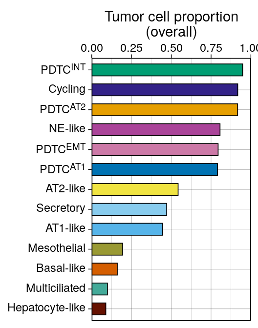
## Figure 3D -- proportion malignant per epithelial state
```{r fig3d-epi-tumor-cell-bar, fig.width = 2.75, fig.height = 3.5}
p4 <- srt_epi@meta.data %>%
  add_count(cell_type_epi, cell_type, name = "n1") %>%
  add_count(cell_type_epi, name = "n2") %>%
  mutate(prop = n1 / n2) %>%
  distinct(cell_type, cell_type_epi, prop, n1, n2) %>%
  # NB: this pipe had been commented out, which left p4 as a data.frame and made
  # the ggsave() below fail -- Figure 3D could not regenerate.
  filter(cell_type == "Tumor Cell") %>%
  ggplot(aes(x = fct_reorder(cell_type_epi, prop, max), y = prop)) +
  geom_col(aes(fill = fct_rev(cell_type_epi)), color = "black", linewidth = 0.3, show.legend = F, width = 0.6) +
  scale_y_continuous(limits = c(0, 1), breaks = seq(0, 1, by = 0.25), expand = c(0, 0)) +
  scale_fill_manual(values = colors$cell_type_epi) +
  guides(
    x = guide_axis(angle = 0, cap = "none", position = "top"),
    y = guide_axis(cap = "none")
  ) +
  labs(fill = "Cell Type", y = "Tumor cell proportion\n(overall)",  x = NULL) +
  scale_x_discrete(labels = label_md) +
  theme_linedraw() +
  # coord_flip(), so the state labels are drawn on the y axis
  theme(axis.text.y = ggtext::element_markdown()) +
  coord_flip()
ggsave(p4, file = here("plots", "epi_tumor_cell_bar.pdf"), width = 2.75, height = 3.5)
p4
```
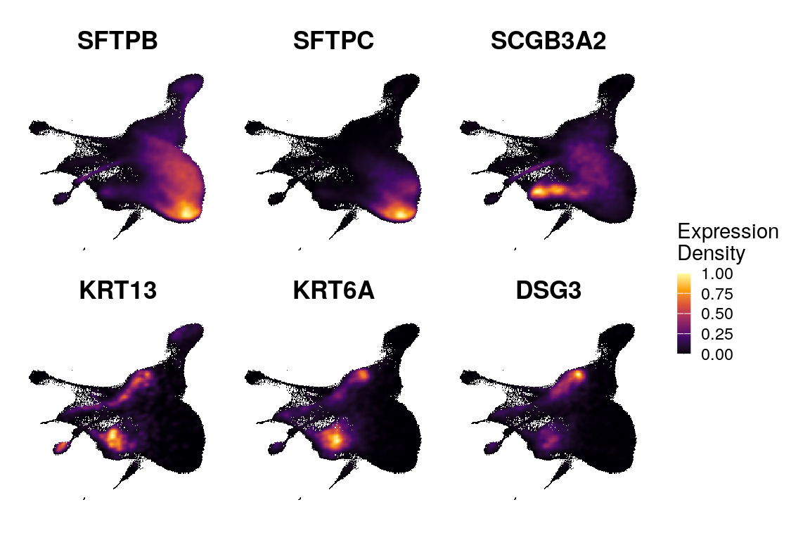
## Figure 3E -- marker expression density on the epithelial UMAP
```{r fig3e-epi-exp-dens, fig.width = 6, fig.height = 4}
glist <- c("SFTPB", "SFTPC", "SCGB3A2", "KRT13", "KRT6A", "DSG3")

x <- Plot_Density_Custom(seurat_object = srt_epi, reduction = "umap", features = glist, viridis_palette = "inferno", joint = F, combine = F) # %>%

names(x) <- glist

res <- map(names(x), .f = function(gene) {
  x[[gene]]$data %>%
    mutate(!!gene := standardize(feature))
})
names(res) <- names(x)

pls <- map(names(res), .f = function(gene) {
  p <- res[[gene]] %>%
    arrange(.data[[gene]]) %>%
    ggplot(aes(x = umap_1, y = umap_2)) +
    scattermore::geom_scattermore(aes(color = .data[[gene]]), pixels = c(256, 256)) +
    # geom_point(aes(color = feature), size = 0.5) +
    scale_color_viridis_c(option = "inferno") +
    labs(title = gene, color = "Density")
  # p <- ggrastr::rasterise(p, dpi = 300)
})

pcomb <- pls %>%
  wrap_plots(nrow = 2, guides = "collect") &
  guides(color = guide_colorbar(keywidth = 0.5, keyheight = 3)) &
  umap_theme() &
  NoAxes() &
  # NoLegend() &
  theme(aspect.ratio = 1, plot.title = element_text(hjust = 0.5, face = "bold")) &
  labs(color = "Expression\nDensity")

pcomb
ggsave(pcomb, filename = here("plots", "epi_exp_dens.pdf"), width = 6, height = 4)
```
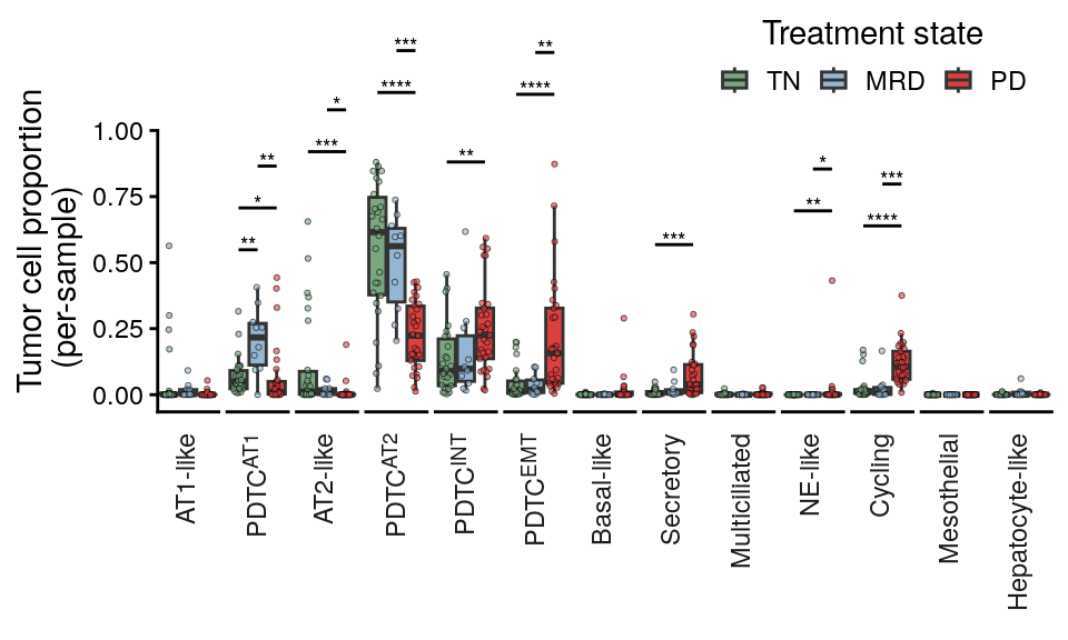
## Figure 3F -- tumor cell proportion per epithelial state
This version is proportion of each pts tumor cells only
```{r fig3f-epi-cluster-proportions, fig.width = 5, fig.height = 3}
use_col <- "cell_type_epi"

df <- srt_epi@meta.data %>%
  filter(cell_type == "Tumor Cell") %>%
  add_count(.data[[use_col]], time_point, sample_id, name = "epi_type_n") %>%
  add_count(sample_id, name = "sample_n") %>%
  mutate(tum_prop = epi_type_n / sample_n) %>%
  distinct(.data[[use_col]], epi_type_n, sample_n, tum_prop, sample_id, time_point) %>%
  tidyr::complete(
    nesting(sample_id, time_point, sample_n),
    .data[[use_col]],
    fill = list(epi_type_n = 0, tum_prop = 0)
  )

# Median of each state by timepoint
meds <- df %>%
  group_by(time_point, .data[[use_col]]) %>%
  summarise(med = median(tum_prop), .groups = "drop") %>%
  pivot_wider(
    names_from = time_point,
    values_from = med)

p_val_df <- df %>%
  group_by(.data[[use_col]]) %>%
  rstatix::wilcox_test(tum_prop ~ time_point, p.adjust.method = "BH") %>%
  rstatix::add_significance() %>%
  filter(p.adj.signif != "ns") %>%
  rstatix::add_xy_position()

pl <- df %>%
  ggplot(aes(x = time_point, y = tum_prop)) +
  geom_boxplot(outliers = F, size = 0.5, aes(fill = time_point), width = 0.9) +
  geom_quasirandom(size = 0.75, alpha = 0.6, color = "black", aes(fill = time_point), stroke = 0.25, pch = 21, width = 0.3, show.legend = F) +
  guides(x = guide_axis(angle = 45)) +
  labs(y = "Tumor cell proportion\n(per-sample)", x = NULL) +
  scale_color_manual(values = colors$time_point) +
  scale_fill_manual(values = colors$time_point) +
  facet_grid(. ~ .data[[use_col]], scales = "free", space = "free", switch = "x",
             labeller = ggplot2::as_labeller(label_md)) +
  ggprism::add_pvalue(p_val_df,
                      tip.length = 0,
                      label = "p.adj.signif",
                      bracket.size = 0.5,
                      label.size = 2.5) +
  theme_classic() +
  scale_y_continuous(breaks = seq(0, 1, by = 0.25), expand = expansion(mult = c(0.05, 0.1))) +
  theme(
    axis.text.x = element_blank(),
    axis.title.y = element_text(hjust = 0.2),
    axis.ticks.x = element_blank(),
    strip.text.x.bottom = ggtext::element_markdown(angle = 90, hjust = 1),
    strip.placement = "outside",
    panel.spacing = unit(1, "mm"),
    strip.clip = "off",
    legend.position = "inside",
    legend.position.inside = c(0.8, 0.9),
    strip.background = element_blank(),
    legend.title.position = "top",
    legend.title = element_text(hjust = 0.5),
    legend.background = element_blank()
  ) +
  labs(fill = "Treatment state") +
  guides(
    x = guide_axis(cap = "none"),
    y = guide_axis(cap = "upper"),
    fill = guide_legend(nrow = 1, keywidth = 0.75, keyheight = 0.75)
  ) +
  coord_cartesian(clip = "off")
ggsave(pl, file = here("plots", "epi_cluster_proportions.pdf"), width = 5, height = 3)
pl
```
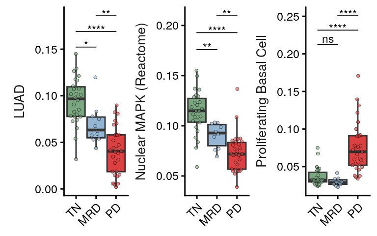
## Figure 3G -- per-specimen signature expression across treatment states
Single table so I can plot select pathways of interest.
```{r}
select_paths <- unique(pth_df$features.plot)
select_paths_name <- unique(pth_df$pathway)

pathway_category_map <- pth_df %>%
  distinct(pathway, feature.groups)

all_sig_summary <- srt_epi@meta.data %>%
  group_by(sample_id, time_point, is_tumor_cell) %>%
  filter(is_tumor_cell) %>%
  summarize(across(all_of(select_paths), ~ mean(.x, na.rm = T))) %>%
  pivot_longer(cols = all_of(select_paths), names_to = "features.plot", values_to = "Score") %>%
  group_by(features.plot) %>%
  mutate(Score_Scaled = scale(Score)[, 1]) %>%
  ungroup() %>%
  mutate(pathway = rename_pathway(features.plot)) %>%
  left_join(pathway_category_map, by = "pathway")
```
Unified statistics: all pairwise Wilcoxon tests across all pathways, single global BH correction.
```{r}
# Compute all pairwise Wilcoxon tests per pathway
all_sig_stats <- all_sig_summary %>%
  group_by(pathway) %>%
  rstatix::wilcox_test(Score ~ time_point) %>%
  ungroup()

# Global BH correction across all tests
all_sig_stats <- all_sig_stats %>%
  mutate(p.adj = p.adjust(p, method = "BH")) %>%
  rstatix::add_significance("p.adj") %>%
  dplyr::rename(p.adj.signif = p.adj.signif)

# Add y positions for plotting (per pathway)
# Order: adjacent comparisons (TN-MRD, MRD-PD) below, spanning (TN-PD) on top
comparison_order <- tibble(
  group1 = c("TN", "MRD", "TN"),
  group2 = c("MRD", "PD", "PD"),
  comp_rank = c(1, 3, 2)
)

all_sig_stats <- all_sig_summary %>%
  group_by(pathway) %>%
  summarize(max_score = max(Score, na.rm = TRUE), .groups = "drop") %>%
  right_join(all_sig_stats, by = "pathway") %>%
  left_join(comparison_order, by = c("group1", "group2")) %>%
  group_by(pathway) %>%
  arrange(pathway, comp_rank) %>%
  mutate(
    y.position = max_score * (1.05 + 0.08 * (comp_rank - 1))
  ) %>%
  ungroup() %>%
  dplyr::select(-comp_rank)

# Save as CSV
write.csv(
  all_sig_stats %>% dplyr::select(pathway, group1, group2, n1, n2, statistic, p, p.adj, p.adj.signif),
  file = here("paper_data", "epi_tumor_signature_pairwise_stats.csv"),
  row.names = FALSE
)
```
```{r fig3g-epi-tumor-boxplot-main, fig.width = 4, fig.height = 2.5}
select_paths_main <- c("LUAD", "Nuclear MAPK (Reactome)", "Proliferating Basal Cell")

stats_main <- all_sig_stats %>%
  filter(pathway %in% select_paths_main) %>%
  mutate(pathway = fct_relevel(pathway, select_paths_main))

p <- all_sig_summary %>%
  filter(pathway %in% select_paths_main) %>%
  ggplot(aes(x = time_point, y = Score)) +
  geom_boxplot(outliers = F, size = 0.5, aes(fill = time_point), width = 0.9) +
  geom_quasirandom(size = 1, alpha = 0.6, color = "black", aes(fill = time_point), stroke = 0.25, pch = 21, width = 0.3) +
  facet_wrap(~ fct_relevel(pathway, select_paths_main), scales = "free", nrow = 1, strip.position = "left") +
  scale_color_manual(values = colors$time_point) +
  scale_fill_manual(values = colors$time_point) +
  coord_cartesian(clip = "off") +
  theme(legend.position = "none", strip.background = element_blank(), strip.text.y = element_text(size = 10), strip.clip = "off", strip.placement = "outside", panel.spacing = unit(0, "mm")) +
  ggpubr::stat_pvalue_manual(stats_main, label = "p.adj.signif", tip.length = 0, label.size = 3, step.increase = 0.03) +
  # scale_y_continuous(expand = expansion(mult = c(0.05, 0.15))) +
  labs(x = NULL, y = NULL) +
  guides(x = guide_axis(angle = 45))
ggsave(p, file = here("plots", "epi_tumor_boxplot_main.pdf"), width = 4, height = 2.5)
p
```
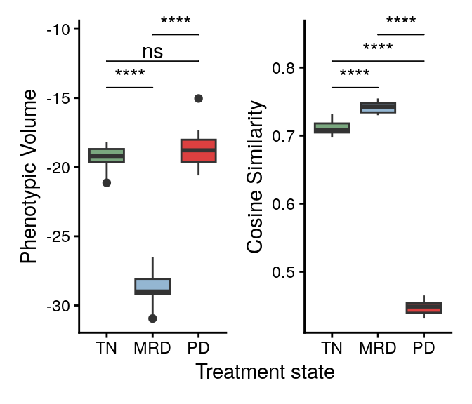
## Figure 3H -- phenotypic volume and cell-cell cosine similarity
Take RPCA cosine distances in each timepoint between cell type pairs. Subsample cells and rerun 1000 times subsampling 1000 cells for each timepoint
```{r}
pseudo_determinant <- function(embedding, tol = 1e-10) {
  # Compute the covariance matrix for the given embedding
  cov_matrix <- cov(embedding)

  # Perform Singular Value Decomposition (SVD) on the covariance matrix
  svd_result <- svd(cov_matrix)

  # Filter out the singular values that are effectively zero (below tolerance)
  nonzero_s <- svd_result$d[svd_result$d > tol]

  # The pseudo-determinant is the product of the nonzero singular values
  pseudo_det <- prod(nonzero_s)

  return(pseudo_det)
}
```
```{r}
sim_out <- here("paper_data", "similarity_results.txt")
# Read the deposited result rather than recomputing it. These are the numbers the
# published Figure 3H was drawn from; recomputing draws a fresh random subsample.
overwrite <- F

if (!file.exists(sim_out) | overwrite) {
  ncores <- 12

  n_subset <- 1000
  n_iter <- 20

  cell_df <- srt@meta.data %>%
    filter(cell_type == "Tumor Cell")

  rpca_mat <- srt@reductions$rnasoup_rpca_integrated@cell.embeddings[cell_df$cell_id, ]

  sim_res <- map(c("TN", "MRD", "PD"), .f = function(tp) {
    res <- pbmcapply::pbmclapply(X = 1:n_iter, mc.cores = ncores, FUN = function(i) {
      ids <- cell_df %>%
        filter(time_point == tp) %>%
        slice_sample(n = n_subset) %>%
        pull(cell_id)

      mat <- rpca_mat[ids, ]

      # mat_norm <- apply(mat, 2, standardize)
      mat_norm <- mat

      # Matrix <- as.matrix(DF)
      sim <- mat_norm / sqrt(rowSums(mat_norm * mat_norm))
      sim <- sim %*% t(sim)

      df <- sim %>%
        reshape2::melt() %>%
        dplyr::filter(Var1 != Var2) %>%
        dplyr::rename(
          "cell1" = "Var1",
          "cell2" = "Var2",
          "similarity" = "value"
        ) %>%
        mutate(iter = i)

      median_sim <- median(df$similarity)

      pheno_vol <- log(pseudo_determinant(mat_norm))

      ret <- data.frame(iter = i, similarity = median_sim, pheno_vol = pheno_vol)

      return(ret)
    }) %>%
      list_rbind() %>%
      mutate(time_point = tp)

    return(res)
  }) %>%
    list_rbind()
  write.table(sim_res, file = sim_out, col.names = T, row.names = F, sep = "\t")
} else {
  sim_res <- read.table(file = sim_out, header = T, sep = "\t")
}

sim_res$time_point <- factor(sim_res$time_point, levels = c("TN", "MRD", "PD"))
```
```{r fig3h-timepoint-similarity-boxplots, fig.width = 3.5, fig.height = 3}
p1 <- sim_res %>%
  ggplot(aes(x = fct_relevel(time_point, "TN", "MRD"), y = similarity)) +
  geom_boxplot(aes(fill = time_point)) +
  labs(y = "Cosine Similarity", x = "Treatment state", fill = "Treatment state") +
  ggpubr::geom_pwc(label = "p.signif", tip.length = 0) +
  scale_fill_manual(values = colors$time_point)

p2 <- sim_res %>%
  ggplot(aes(x = fct_relevel(time_point, "TN", "MRD"), y = pheno_vol)) +
  geom_boxplot(aes(fill = time_point)) +
  labs(y = "Phenotypic Volume", x = "Treatment state", fill = "Treatment state") +
  ggpubr::geom_pwc(label = "p.signif", tip.length = 0) +
  scale_fill_manual(values = colors$time_point)

pcomb <- p2 + p1 + plot_layout(guides = "collect", axes = "collect") &
  NoLegend() &
  coord_cartesian(clip = "off")
ggsave(pcomb, file = here("plots", "timepoint_similarity_boxplots.pdf"), width = 3.5, height = 3)
pcomb
```
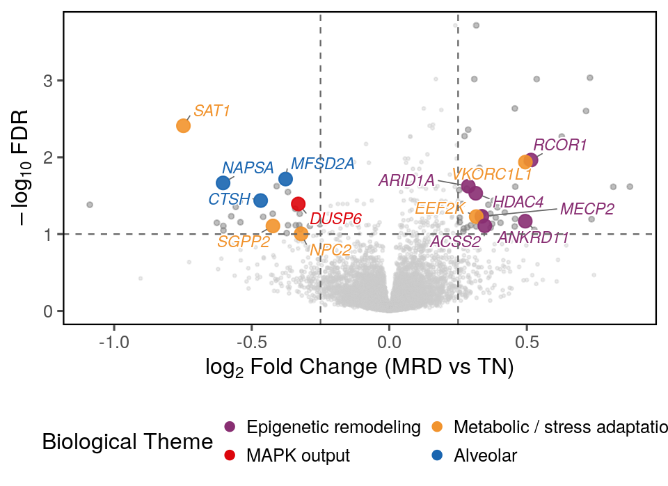
## Figure 3I -- MRD vs TN differential expression volcano
The mixed-model fits behind Figure 3I and S8 are shipped in `paper_data/`, since
refitting them takes hours. Delete the file to refit.
```{r flashmm-cache}
flashmm_stale <- function(fit_f, obj_f = NULL) !file.exists(fit_f)
```
```{r}
library(FLASHMM)
library(cluster)

fit_f <- here("paper_data", "flashmm_tumor_fit.rds")
if (!flashmm_stale(fit_f, here("paper_data", "egfr_epi.rds"))) {
  cli::cli_alert("Loading existing FLASHMM model fit for tumor cells...")
  fit <- readRDS(fit_f)
} else {
  cli::cli_alert("Fitting FLASHMM model for tumor cells...")
  Y <- srt_tum[["RNAsoup"]]$data %>%
    as(., "dgCMatrix")

  # Only keep genes expressed in at least 5% of the subsetted cells
  keep_genes <- rowSums(Y > 0) >= (0.05 * ncol(Y))
  keep_genes <- names(which(keep_genes))
  Y <- Y[keep_genes, ]

  metadata <- srt_tum@meta.data
  metadata$sample_id <- factor(metadata$sample_id)
  metadata$time_point <- factor(metadata$time_point, levels = c("TN", "MRD", "PD"))

  X <- model.matrix(~ 0 + log(nCount_RNA) + time_point, data = metadata)

  Z <- model.matrix(~ 0 + sample_id, data = metadata)
  d <- ncol(Z)

  max.iter <- 100
  epsilon <- 1e-5

  ss <- sslmm(X, Y, Z)
  rm(X, Y, Z)

  fit <- lmm(ss$XX, ss$XY, ss$ZX, ss$ZY, ss$ZZ,
    Ynorm = ss$Ynorm, n = ss$n, d = d,
    max.iter = max.iter, epsilon = epsilon
  )
  saveRDS(fit, file = fit_f)
}
```
```{r}
fit <- readRDS(fit_f)

epsilon <- 1e-5
fdr_cutoff <- 0.1
lfc_cutoff <- 0.25

# Check convergence
convg <- apply(abs(fit$dlogL), 2, max) < epsilon
cat("Converged:", sum(convg), "out of", length(convg), "genes\n")
# Helper to run a single contrast and return a tidy data.frame
run_contrast <- function(fit, contrast_str, label) {
  ct <- contrast.matrix(
    contrast = setNames(contrast_str, label),
    model.matrix.names = rownames(fit$coef)
  )
  res <- lmmtest(fit, contrast = ct)
  t_stat <- res[, 2]
  # Recompute two-sided p-values from t-statistics using log-scale normal CDF.
  # pnorm(..., log.p = TRUE) stays finite for extreme t-statistics that would
  # otherwise underflow to p = 0 with the standard 2*pnorm() call.
  log_p <- pnorm(abs(t_stat), lower.tail = FALSE, log.p = TRUE) + log(2)
  data.frame(
    gene = colnames(fit$coef),
    coef = res[, 1],
    t = t_stat,
    p = pmax(exp(log_p), .Machine$double.xmin),  # floor at ~2.2e-308
    neg_log10_p = -log_p / log(10),              # precise -log10(p), never Inf
    row.names = NULL
  ) %>%
    mutate(FDR = p.adjust(p, method = "fdr")) %>%
    arrange(p)
}

mrd_tn_results <- run_contrast(fit, "time_pointMRD - time_pointTN", "MRD_vs_TN")
pd_tn_results <- run_contrast(fit, "time_pointPD - time_pointTN", "PD_vs_TN")
pd_mrd_results <- run_contrast(fit, "time_pointPD - time_pointMRD", "PD_vs_MRD")

# Flag significant genes
mrd_tn_results$sig <- (mrd_tn_results$FDR < fdr_cutoff) & (abs(mrd_tn_results$coef) > lfc_cutoff)
pd_tn_results$sig <- (pd_tn_results$FDR < fdr_cutoff) & (abs(pd_tn_results$coef) > lfc_cutoff)
pd_mrd_results$sig <- (pd_mrd_results$FDR < fdr_cutoff) & (abs(pd_mrd_results$coef) > lfc_cutoff)

# Merge into unified results table
all_results <- mrd_tn_results[, c("gene", "coef", "FDR", "sig")] %>%
  dplyr::rename(coef.mrd_tn = coef, FDR.mrd_tn = FDR, sig.mrd_tn = sig) %>%
  left_join(
    pd_tn_results[, c("gene", "coef", "FDR", "sig")] %>%
      dplyr::rename(coef.pd_tn = coef, FDR.pd_tn = FDR, sig.pd_tn = sig),
    by = "gene"
  ) %>%
  left_join(
    pd_mrd_results[, c("gene", "coef", "FDR", "sig")] %>%
      dplyr::rename(coef.pd_mrd = coef, FDR.pd_mrd = FDR, sig.pd_mrd = sig),
    by = "gene"
  )

# Test variance components (sample random effect)
i_var <- grep("var1", rownames(fit$theta))
z_var <- fit$theta[i_var, ] / fit$se.theta[i_var, ]
p_var <- pnorm(z_var, lower.tail = FALSE)
cat(
  "Genes with significant sample random effect (Bonferroni):",
  sum(p_var < 0.05 / length(p_var)), "\n"
)
```
```{r fig3i-mrd-vs-tn-volcano-plot-highlighted-genes, fig.width=5.5/1.1, fig.height = 4/1.1}
library(ggplot2)
library(ggrepel)
library(dplyr)

x <- (all_results %>%
       filter(FDR.mrd_tn < 0.1 & abs(coef.mrd_tn) > 0.25))
x <- split(x$gene, sign(x$coef.mrd_tn))

highlight_categories <- list(
  "Epigenetic remodeling"         = c("HDAC4", "MECP2", "RCOR1", "ANKRD11", "ARID1A", "ACSS2"),
  "Metabolic / stress adaptation" = c("EEF2K", "SAT1", "SGPP2", "NPC2", "VKORC1L1"),
  "MAPK output"                   = c("DUSP6"),
  "Alveolar"             = c("NAPSA", "MFSD2A", "CTSH")
)

highlight_df <- stack(highlight_categories) %>%
  setNames(c("gene", "highlight_category"))

category_colors <- c(
  "Epigenetic remodeling"         = "#882E72",
  "Metabolic / stress adaptation" = "#F1932D",
  "MAPK output"                   = "#DC050C",
  "Alveolar"             = "#1965B0",
  "NS"                            = "grey80"
)
# Dropped: PIGR (secretory + sub-threshold), CAPN8 (GI calpain), RNASE1 (myeloid/ambient),
#          DUSP1 & HLA-DRA (sub-threshold). NFKBIA/CEBPD = NF-kB/stress IEGs, not MAPK — leave NS.
# Optional exploratory (GSEA-concordant, interpretation thin): "Glycan/proteoglycan" = c("EXT1","GPC4")

# Prepare plotting data
plot_df <- all_results %>%
  mutate(
    neg_log10_fdr = -log10(FDR.mrd_tn),
    log2FC = coef.mrd_tn
  ) %>%
  left_join(highlight_df, by = "gene") %>%
  mutate(
    # Assign significance category for non-highlighted genes
    sig = case_when(
      !is.na(highlight_category) ~ highlight_category,
      FDR.mrd_tn < 0.1 & abs(log2FC) > 0.25 ~ "Significant (unlabeled)",
      TRUE ~ "NS"
    ),
    # Flag genes to label
    label_gene = ifelse(!is.na(highlight_category), gene, NA_character_)
  )

# Set factor order so highlighted points are plotted on top
plot_df$sig <- factor(plot_df$sig,
                      levels = c("NS", "Significant (unlabeled)",
                                 names(category_colors)[1:4]))

lab_sz = 3

# Plot
p <- ggplot(plot_df, aes(x = log2FC, y = neg_log10_fdr)) +
  # Background non-significant points
  geom_point(data = filter(plot_df, sig == "NS"),
             color = "grey80", size = 0.5, alpha = 0.4) +
  # # Significant but not highlighted
  geom_point(data = filter(plot_df, sig == "Significant (unlabeled)"),
             color = "grey50", size = 1.0, alpha = 0.5) +
  # Highlighted category points

  geom_point(data = filter(plot_df, sig %in% names(highlight_categories)),
             aes(color = sig), size = 3, alpha = 0.9) +
  # Labels - left side genes (negative FC)
  geom_text_repel(
    data = filter(plot_df, !is.na(label_gene)),
    aes(label = label_gene, color = sig),
    size = lab_sz,
    fontface = "italic",
    max.overlaps = Inf,
    bg.colour = "white",
    bg.r = 0.1,
    box.padding = 0.3,
    point.padding = 0.2,
    segment.color = "grey40",
    segment.size = 0.3,
    min.segment.length = 0,
    show.legend = FALSE,
    direction = "both",
    force = 2
  ) +
  # Scales
 scale_color_manual(
    values = c(category_colors, "Significant (unlabeled)" = "grey50"),
    breaks = names(category_colors)[1:5],  # Only show 5 categories in legend
    name = "Biological Theme"
  ) +
  # Cutoff lines
  geom_hline(yintercept = -log10(0.1), linetype = "dashed", color = "grey40", linewidth = 0.4) +
  geom_vline(xintercept = c(-0.25, 0.25), linetype = "dashed", color = "grey40", linewidth = 0.4) +
  labs(
    x = expression(log[2]~"Fold Change (MRD vs TN)"),
    y = expression(-log[10]~"FDR")
  ) +
  theme_few(base_size = 12) +
  guides(
    color = guide_legend(override.aes = list(size = 2, alpha = 1),
                         keywidth = 0, keyheight = 0, nrow = 2, byrow = TRUE)
  ) +
  theme(
    panel.border = element_rect(color = "black", fill = NA, linewidth = 0.8),
    panel.grid.minor = element_blank(),
    legend.position = "bottom",
    plot.title = element_text(face = "bold", size = 13),
    plot.subtitle = element_text(size = 10, color = "grey30")
  )
ggsave(p, file = here("plots", "MRD_vs_TN_volcano_plot_highlighted_genes.pdf"), width = 5.5/1.1, height = 4/1.1)
p
```
# Figure S6 -- Epithelial cell state annotation
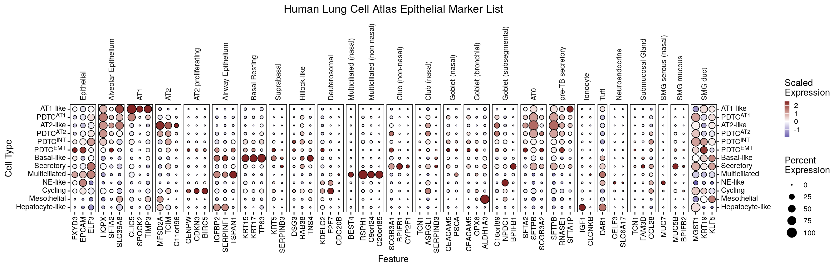
## Figure S6A -- HLCA marker dot plot across epithelial states
```{r figs6a-hlca-marker-dotplot, fig.width = 14, fig.height = 4.5}
dp <- DotPlotter(md_epi_states(srt_epi), features = markers$epi_markers_hlca, group.by = "cell_type_epi", cluster_groups = F, rotate_y_strip = T)
dp_f <- dp + theme(panel.spacing = unit(1, "mm")) +
  guides(y.sec = guide_axis()) +
  labs(title = "Human Lung Cell Atlas Epithelial Marker List") +
  theme(plot.title = element_text(hjust = 0.5),
        axis.text.y = ggtext::element_markdown(),
        # Both sides explicitly: y.sec draws axis.text.y.right, which the active theme sets
        # itself, so it does not inherit and the labels come out as literal <sup> tags.
        axis.text.y.right = ggtext::element_markdown(hjust = 0),
        strip.text.y.left = ggtext::element_markdown())
dp_f
ggsave(dp_f, file = here("plots", "hlca_marker_dotplot.pdf"), width = 14, height = 4.5)
```
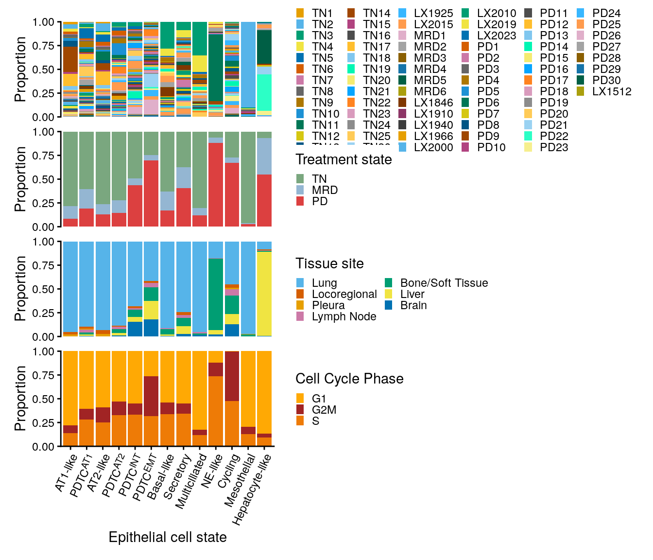
## Figure S6B-E -- epithelial state composition by patient, state, site, phase
```{r figs6be-epi-type-feature-proportions, fig.width = 7, fig.height = 6}
p1 <- srt_epi@meta.data %>%
  ggplot(aes(x = cell_type_epi)) +
  geom_bar(aes(fill = sample_id), position = "fill") +
  scale_fill_manual(values = colors$sample_id) +
  labs(fill = "Patient", y = "Proportion") +
  guides(fill = guide_legend(keywidth = 0.5, keyheight = 0.5, ncol = 6))

p2 <- srt_epi@meta.data %>%
  ggplot(aes(x = cell_type_epi)) +
  geom_bar(aes(fill = site_of_tissue_simple), position = "fill") +
  scale_fill_manual(values = colors$site_of_tissue_simple) +
  labs(fill = "Tissue site", y = "Proportion") +
  guides(fill = guide_legend(keywidth = 0.5, keyheight = 0.5, ncol = 2))

p3 <- srt_epi@meta.data %>%
  ggplot(aes(x = cell_type_epi)) +
  geom_bar(aes(fill = time_point), position = "fill") +
  scale_fill_manual(values = colors$time_point) +
  guides(x = guide_axis(angle = 45)) +
  labs(fill = "Treatment state", y = "Proportion") +
  guides(fill = guide_legend(keywidth = 0.5, keyheight = 0.5))

p4 <- srt_epi@meta.data %>%
  filter(sample_has_tumor) %>%
  # filter(!grepl("PD9", cell_type_epi)) %>%
  add_count(cell_type_epi, cell_type, name = "n1") %>%
  add_count(cell_type_epi, name = "n2") %>%
  mutate(prop = n1 / n2) %>%
  distinct(cell_type, cell_type_epi, prop) %>%
  filter(cell_type == "Tumor Cell") %>%
  ggplot(aes(x = cell_type_epi, y = prop)) +
  geom_col(aes(fill = fct_rev(cell_type)), show.legend = F) +
  geom_hline(yintercept = seq(0.25, 1, by = 0.25), alpha = 0.6, linetype = "dashed", color = "grey50", linewidth = 0.5) +
  scale_y_continuous(limits = c(0, 1), breaks = seq(0, 1, by = 0.25)) +
  scale_fill_manual(values = colors$cell_type) +
  labs(y = "Proportion\n(tumor cells)")

p5 <- srt_epi@meta.data %>%
  ggplot(aes(x = cell_type_epi)) +
  geom_bar(aes(fill = Phase), position = "fill") +
  scale_fill_manual(values = colors$Phase) +
  guides(x = guide_axis(angle = 45)) +
  labs(fill = "Cell Cycle Phase", y = "Proportion") +
  guides(fill = guide_legend(keywidth = 0.5, keyheight = 0.5))

gap_size <- 2

pcomb <- wrap_plots(
  # free(p1, type = "space", side = "r"),
  p1 + theme(plot.margin = margin(t = 4, r = 2, b = gap_size, l = 2, "mm")),
  free(p3 + theme(plot.margin = margin(t = gap_size, r = 2, b = gap_size, l = 2, "mm")), type = "space", side = "r"),
  free(p2 + theme(plot.margin = margin(t = gap_size, r = 2, b = gap_size, l = 2, "mm")), type = "space", side = "r"),
  # p2,
  free(p5 + theme(plot.margin = margin(t = gap_size, r = 2, b = gap_size, l = 2, "mm")), type = "space", side = "r"),
  # free(p4 + theme(plot.margin = margin(t = gap_size, r = 2, b = 2, l = 4, "mm")), type = "space", side = "l"),
  ncol = 1, axes = "collect_x"
) &
  guides(
    x = guide_axis(angle = 65, cap = "none"),
    y = guide_axis(cap = "both")
  ) &
  scale_y_continuous(expand = c(0, 0)) &
  scale_x_discrete(labels = label_md) &
  labs(x = "Epithelial cell state") &
  theme(axis.text.x = ggtext::element_markdown(angle = 65, hjust = 1)) &
  coord_cartesian(clip = "off")
ggsave(pcomb, file = here("plots", "epi_type_feature_proportions.pdf"), width = 7, height = 7)
pcomb
```
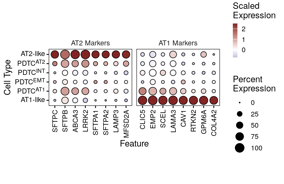
## Figure S6F -- canonical AT1/AT2 markers across AT-like and PDTC states
```{r figs6f-dotplot-at12-epi-states, fig.width = 5, fig.height = 3.25}
alveolar_markers <- list(
  AT1 = c("AGER", "PDPN", "CAV1", "HOPX", "CLIC5",
          "TIMP3", "CAV1"),
  AT2 = c("SFTPB", "SFTPC", "SFTPA1", "SFTPD", "ABCA3",
          "NAPSA", "LAMP3", "SLC34A2", "ETV5", "LRRK2", ""),
  Pan_epithelial = c("NKX2-1"),
  Secretory_Club = c("SCGB3A1", "SCGB3A2"),
  Other <- c("ABCC3", "CAMK1D", "FGF13", "LRRK2", "LGR4")
)

gene_panel <- list(
  "AT2 Markers"         = c("SFTPC", "SFTPB", "ABCA3", "LRRK2", "SFTPA1", "SFTPA2", "LAMP3", "MFSD2A"),
  # "PDTC Plasticity"    = c("RUNX1", "LGR4", "TOX3", "RAD51B", "SEPT9", "ABCC3"),
  "AT1 Markers"          = c("CLIC5", "EMP2", "SCEL", "LAMA3", "CAV1", "RTKN2", "GPM6A", "COL4A2")
)

p <- DotPlotter(md_epi_states(srt_epi),
                group.by = "cell_type_epi",
                cluster_feats = F,
                cluster_groups = F,
                features = gene_panel,
                subset_types = label_md(c("AT2-like", "PDTC^AT2", "PDTC^INT", "PDTC^EMT", "PDTC^AT1", "AT1-like")))
pfinal <- p +
  theme(plot.margin = margin(t = 45, r = 5, b = 45, l = 5),
        axis.text.y = ggtext::element_markdown(),
        strip.text.y.left = ggtext::element_markdown())
pfinal
ggsave(pfinal, file = here("plots", "dotplot_at12_epi_states.pdf"), width = 5, height = 3.25)
```
# Figure S7 -- Tumor cell signatures and IHC data
## Figure S7A -- the 36 remaining tumor-cell signatures
```{r figs7a-epi-sig-tumor-specific-boxplots-supplement, fig.width = 8, fig.height = 9}
# Supplemental: exclude main 3, order by heatmap category
select_paths_supp <- setdiff(select_paths_name, select_paths_main)

# Order by category (pth_cat_order) then by pth_order within each category
supp_order <- pathway_category_map %>%
  filter(pathway %in% select_paths_supp) %>%
  distinct(pathway, feature.groups) %>%
  mutate(
    cat_rank = match(feature.groups, pth_cat_order),
    pth_rank = match(pathway, pth_order)
  ) %>%
  arrange(cat_rank, pth_rank) %>%
  pull(pathway)

stats_supp <- all_sig_stats %>%
  filter(pathway %in% select_paths_supp) %>%
  mutate(pathway = factor(pathway, levels = supp_order))

p <- all_sig_summary %>%
  filter(pathway %in% select_paths_supp) %>%
  mutate(pathway = factor(pathway, levels = supp_order)) %>%
  ggplot(aes(x = time_point, y = Score)) +
  geom_boxplot(outliers = F, size = 0.5, aes(fill = time_point), width = 0.9) +
  geom_quasirandom(size = 1, alpha = 0.6, color = "black", aes(fill = time_point),
                   stroke = 0.25, pch = 21, width = 0.3, show.legend = F) +
  facet_wrap2(~pathway, scales = "free_y", strip.position = "left", ncol = 6, remove_labels = "x") +
  scale_fill_manual(values = colors$time_point) +
  coord_cartesian(clip = "off") +
  theme(legend.position = "top", strip.background = element_blank(), strip.clip = "off", strip.placement = "outside",
        panel.border = element_rect(fill = NA, color = "black", linewidth = 0.25),
        axis.line = element_blank()) +
  ggpubr::stat_pvalue_manual(stats_supp, label = "p.adj.signif", tip.length = 0, label.size = 2.5) +
  scale_y_continuous(expand = expansion(mult = c(0.05, 0.1)),
                                        breaks = scales::breaks_pretty(n = 3)) +
  labs(x = NULL, y = "Signature scores", fill = "Treatment state") +
  guides(x = guide_axis(angle = 45))
ggsave(p, file = here("plots", "epi_sig_tumor_specific_boxplots_supplement.pdf"), width = 8, height = 9)
p
```
## Figure S7B -- IHC scoring categories by treatment state
```{r figs7b-ihc-score-cat-barplots, fig.width = 5, fig.height = 3}
score_cat_cols <- c("Negative" = "#A8C5E2",
             "Low" = "#D4A574",
             "Medium" = "#8B6914",
             "High" = "#4A2800")

sel_stains <- c("TTF_1", "NAPSIN_A", "P40", "DUSP6")

## Add counts for each category in the x labels and save pdf

p <- ihc_long %>%
  add_count(time_point, gene, stain_loc, wt = !is.na(score_cat), name = "n_stains") %>%
  filter(gene %in% sel_stains) %>%
  filter_out(gene == "DUSP6" & stain_loc == "Nuclear") %>%
  mutate(time_point = factor(time_point, levels = c("TN", "MRD", "PD"))) %>%
  mutate(time_point_lab = fct_reorder(paste0(time_point, "\n(n=", n_stains, ")"), as.integer(time_point))) %>%
  ggplot(aes(x = time_point_lab)) +
  geom_bar(aes(fill = score_cat), color = "black", position = "fill", na.rm = TRUE) +
  # scale_color_manual(values = colors$histology_predominant_short) +
  scale_fill_manual(values = score_cat_cols) +
  scale_y_continuous(expand = c(0, 0)) +
  guides(fill = guide_legend(reverse = T, keywidth = 0.5, keyheight = 0.5)) +
  theme(strip.background = element_blank(),
        strip.clip = "off",
        legend.position = "bottom") +
  coord_cartesian(clip = "off") +
  facet_nested(. ~ fct_relevel(gene, sel_stains), scales = "free", space = "free") +
  # Reviewer #1 C7: axis reads "treatment state", matching the Figure S7 legend.
  labs(x = "Treatment state", y = "IHC Score",
       fill = "Score")
ggsave(p, file = here("plots", "ihc_score_cat_barplots.pdf"), width = 5.5, height = 3)
p
```
# Figure S8 -- Gene-set enrichment and tumor-cell library quality
## Figure S8A -- KEGG GSEA of the MRD vs TN program
```{r}
library(clusterProfiler)
library(enrichplot)
library(ReactomePA)
id_map <- bitr(all_results$gene,
  fromType = "SYMBOL",
  toType = "ENTREZID", OrgDb = "org.Hs.eg.db", drop = F
)

all_results$gene_entrez <- id_map$ENTREZID[match(all_results$gene, id_map$SYMBOL)]

tn_v_mrd_list_entrez <- all_results %>%
  dplyr::filter(!is.na(gene_entrez)) %>%
  arrange(desc(coef.mrd_tn)) %>%
  dplyr::select(gene_entrez, coef.mrd_tn) %>%
  deframe()

tn_v_mrd_list <- all_results %>%
  # dplyr::filter(!is.na(gene_entrez)) %>%
  arrange(desc(coef.mrd_tn)) %>%
  dplyr::select(gene, coef.mrd_tn) %>%
  deframe()

# Read the deposited result rather than recomputing it. These are the numbers the
# published Figure S8A was drawn from. Recomputing is not reproducible: gseKEGG() scores
# by permutation, and it pulls current gene-set definitions from rest.kegg.jp at run time,
# so both the statistics and the sets themselves move between renders. Set overwrite to
# TRUE to recompute -- seeded, but against whatever KEGG serves that day.
kegg_out <- here("paper_data", "kegg_gsea_mrd_vs_tn.csv")
overwrite <- FALSE

if (overwrite || !file.exists(kegg_out)) {
  set.seed(42)
  gse_kegg <- gseKEGG(geneList = tn_v_mrd_list_entrez,
                 organism     = 'hsa',
                 pvalueCutoff = 0.05,
                 seed         = TRUE,
                 verbose      = FALSE)
  # OrgDb as a string, not a bare symbol: load_OrgDb() resolves it out of the namespace,
  # so this no longer depends on some earlier call having attached org.Hs.eg.db.
  gse_kegg <- setReadable(gse_kegg, OrgDb = "org.Hs.eg.db", keyType = "ENTREZID")
  write.csv(gse_kegg@result, kegg_out, row.names = FALSE)
}

kegg_result <- read.csv(kegg_out)
```
```{r figs8a-kegg-gsea-dotplot, fig.width = 7, fig.height = 4}
library(dplyr)
library(ggplot2)

# Step 1: Filter disease/infection/autoimmune labels
disease_keywords <- c("Coronavirus", "HIV", "Hepatitis", "Influenza",
                      "Herpes", "Epstein", "Measles", "Pertussis",
                      "Leishmaniasis", "Malaria", "Tuberculosis",
                      "Staphylococcus", "Shigellosis", "Salmonella",
                      "Yersinia", "Legionellosis", "Vibrio",
                      "Prion", "Amoebiasis", "Toxoplasmosis",
                      "Kaposi", "leukemia virus", "Escherichia",
                      "trypanosomiasis", "Type I diabetes",
                      "Autoimmune thyroid", "Graft-versus-host",
                      "Allograft rejection", "Asthma",
                      "Systemic lupus", "Inflammatory bowel",
                      "Rheumatoid arthritis", "Diabetic cardiomyopathy",
                      "Parkinson", "Amyotrophic lateral", "Alzheimer",
                      "Atherosclerosis", "neurodegeneration")

kegg_filtered <- kegg_result %>%
  filter(!grepl(paste(disease_keywords, collapse = "|"), Description, ignore.case = TRUE)) %>%
  filter(setSize < 500 & setSize > 15)

# Step 2: Remove redundant pathways (same ETC/OXPHOS gene sets)
kegg_final <- kegg_filtered %>%
  filter(!(Description %in% c("Cardiac muscle contraction", "Thermogenesis")))

# Step 3: Order by NES
kegg_final <- kegg_final %>%
  arrange((NES)) %>%
  mutate(Description = factor(Description, levels = Description))

# Step 4: Plot
p_dot <- ggplot(kegg_final, aes(x = NES, y = Description)) +
  geom_segment(aes(x = 0, xend = NES, yend = Description),
               color = "grey70", linewidth = 0.3) +
  geom_point(aes(size = setSize, color = -log10(p.adjust)), stroke = 0.4) +
  scale_color_gradient(low = "#fdae61", high = "#b2182b",
                       name = expression(-log[10]~"FDR")) +
  scale_size_continuous(range = c(3, 7), name = "Gene Set Size") +
  geom_vline(xintercept = 0, linetype = "dashed", color = "grey30") +
  labs(x = "Normalized Enrichment Score (NES)",
       y = NULL,
       title = "GSEA: KEGG Pathways (MRD vs TN)") +
  theme_few(base_size = 11) +
  theme(
    panel.border = element_rect(color = "black", fill = NA, linewidth = 0.6),
    panel.grid.major.y = element_line(color = "grey92"),
    panel.grid.minor = element_blank(),
    legend.position = "right",
    plot.title = element_text(face = "bold")
  )
p_dot
ggsave(p_dot, file = here("plots", "kegg_gsea_dotplot.pdf"), width = 7, height = 4)
```
## Figure S8B -- per-sample tumor-cell library quality metrics
```{r figs8b-qc-tumor-cells-violins, fig.width = 6.5, fig.height = 3}
srt_tum <- scCustomize::Add_Cell_Complexity(srt_tum, overwrite = T)

srt_tum$log10_counts <- log10(srt_tum$nCount_RNA)
srt_tum$log10_genes <- log10(srt_tum$nFeature_RNA)

p <- plot_feats(srt_tum, feats = c("log10_counts", "log10_genes", "log10GenesPerUMI", "percent_ribo"), group.by = "time_point", sample_col = "sample_id", min_cells = 20)

# Helper: auto log10-scale for pre-transformed data
scale_y_log10_pretransformed <- function(n = 7) {
  scale_y_continuous(
    breaks = function(lims) {
      brks <- scales::breaks_log(n = n)(10^lims)
      log10(brks)
    },
    labels = function(brks) scales::comma(10^brks)
  )
}

pcomb <- (p$log10_counts + labs(y = "UMI counts", title = NULL) + scale_y_log10_pretransformed()) +
  (p$log10_genes + labs(y = "Genes detected", title = NULL) + scale_y_log10_pretransformed()) +
  (p$log10GenesPerUMI + labs(y = "Library complexity\n(log10GenesPerUMI)", title = NULL)) +
  (p$percent_ribo + labs(y = "Ribosomal transcript percentage", title = NULL)) +
  plot_layout(nrow = 1, guides = "collect", axes = "collect_x") &
  scale_fill_manual(values = colors$time_point) &
  labs(x = "Treatment state")
ggsave(pcomb, file = here("plots", "qc_tumor_cells_violins.pdf"), width = 6.5, height = 3)
pcomb
```