---
title: "Figure 5 and S10 -- dynamics of lineage plasticity"
author: "Matthew Zatzman"
execute:
warning: false
error: false
format:
html:
code-fold: true
code-tools: true
toc: true
---
Figure 5 and Supplementary Figure S10 (histotime analysis).
"leaning" survives in the S10C-G cached filenames and factor levels only -- the
manuscript term is **lineage-primed**.
Run `00_download_convert.qmd` first to build `paper_data/`.
{{< include _setup.qmd >}}
# Load data
The epithelial and histotime objects carry every panel here.
```{r load}
# L'Ecuyer-CMRG so forked mclapply workers get reproducible streams.
RNGkind("L'Ecuyer-CMRG")
set.seed(42)

db <- load_project(objects = c("epi", "histo"))

srt_epi <- db$srt_epi
srt_ti  <- db$srt_ti

# Grey all-timepoint background for S10I
df_raw_background <- FetchData(srt_epi, vars = c("time_point", "is_tumor_cell", "cell_type",
                                                 "umap_1", "umap_2")) %>%
  dplyr::rename("UMAP1" = "umap_1", "UMAP2" = "umap_2") %>%
  filter(is_tumor_cell)
```
## Trajectory objects
The Slingshot fit and the tradeSeq GAMs are not part of the deposited objects -- the h5ad
schema has nowhere to put them -- so they travel as their own files.
```{r trajectory}
library(slingshot)
library(tradeSeq)

sce_ti  <- readRDS(here("paper_data", "slingshot_sce.rds"))
sce_gam <- readRDS(here("paper_data", "sce_gam.rds"))

sce_ti$pseudotime <- rowMeans(slingPseudotime(sce_ti), na.rm = TRUE)

# Fitted curves in the PCA_GENES embedding, for the Fig 5A trajectory overlays.
embedded <- slingCurves(embedCurves(sce_ti, "PCA_GENES"))
curves_df <- purrr::map(seq_along(embedded), function(i) {
  df <- as.data.frame(embedded[[i]]$s[embedded[[i]]$ord, ])
  df$lineage <- i
  df
}) %>%
  bind_rows() %>%
  mutate(lineage = factor(lineage, levels = c(1, 2), labels = c("SCLC", "LUSC")))

# The fitted GAM curves for every gene, read by the Fig 5B/5C panels below.
ysmooth_df_full <- predictSmooth(models = sce_gam, gene = rownames(sce_gam),
                                 nPoints = 100, tidy = TRUE) %>%
  mutate(log_counts = log1p(yhat)) %>%
  mutate(lineage = factor(lineage, levels = c(2, 1), labels = c("LUSC", "SCLC"))) %>%
  group_by(gene, lineage) %>%
  mutate(pseudotime_rank = 1:n(),
         time_scaled = standardize(pseudotime_rank)) %>%
  ungroup() %>%
  group_by(gene) %>%
  mutate(log_counts_scaled = scale(log_counts)[, 1],
         log_counts_standardized = standardize(log_counts)) %>%
  ungroup()
```
```{r pathways}
pathways <- read.table(here("paper_data", "egfr_pathways_annotations.txt"),
                       header = TRUE, sep = "\t")
mapk_paths <- filter(pathways, category == "MAPK")$pathway
tum_paths  <- c("LUAD", "LUSC", "SCLC")

rename_sigs <- function(df) {
  df$pathway[df$pathway == "LUAD_GIRARD"] <- "LUAD"
  df$pathway[df$pathway == "LUSC_GIRARD"] <- "LUSC"
  df$pathway[df$pathway == "SCLC_CCLE"]   <- "SCLC"
  df
}
pathways <- rename_sigs(pathways)

pathways_v2 <- read.table(here("paper_data", "egfr_pathways_v2.txt"),
                          header = TRUE, sep = "\t")
pathways_v2_t2g <- pathways_v2 %>% dplyr::relocate(pathway, Gene)

pathways_full <- bind_rows(
  pathways_v2,
  read.csv(here("paper_data", "tirosh_mps_67_natcan_2025.csv")) %>%
    dplyr::rename(pathway = Geneset) %>%
    dplyr::select(pathway, Gene)
) %>% rename_sigs()
```
## Standardize scores
```{r derived-columns}
# Deposited, not derived. Asserted rather than recomputed, so a deposit that ever stops
# carrying them fails here loudly instead of somewhere downstream in a panel.
stopifnot(
  is.numeric(srt_ti$Histotime_s), is.numeric(srt_ti$lineage_probability2),
  !anyNA(srt_ti$Histotime_s), !anyNA(srt_ti$lineage_probability2)
)

# The rescaled lineage and MAPK scores the Fig 5A trajectory panels plot.
# trim = c(0, 1) is the full range, so this is a plain rescale to [0, 1].
trim_v <- c(0, 1)
srt_ti$LUAD_s <- standardize(srt_ti$LUAD_GIRARD, trim = trim_v)
srt_ti$LUSC_s <- standardize(srt_ti$LUSC_GIRARD, trim = trim_v)
srt_ti$SCLC_s <- standardize(srt_ti$SCLC_CCLE,   trim = trim_v)
srt_ti$MAPK_s <- standardize(
  srt_ti$REACTOME_MAPK_TARGETS_NUCLEAR_EVENTS_MEDIATED_BY_MAP_KINASES, trim = trim_v)
stopifnot(all(c("Histotime_s", "LUAD_s", "LUSC_s", "SCLC_s", "MAPK_s") %in%
              colnames(srt_ti@meta.data)))

# The epithelial object carries the same two columns already, NA off the trajectory --
# so the back-join this chunk used to do is redundant. Same check it used to end on.
stopifnot(sum(!is.na(srt_epi$lineage_probability2)) == ncol(srt_ti))
```
# Figure 5 -- Dynamics of lineage plasticity
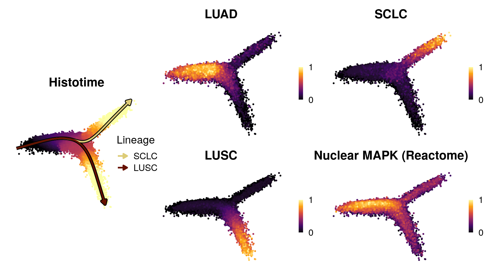
## Figure 5A -- histotime trajectory of tumor cells
```{r}
library(slingshot); library(tradeSeq)
```
Quick check what this would look like over cell types
```{r fig5a-psuedotime-traj, fig.width = 9, fig.height = 5}
library(ggnewscale)

p_list <- FeaturePlot(srt_ti, features = c("Histotime_s", "LUAD_s", "LUSC_s", "SCLC_s", "MAPK_s"), reduction = "histotime", raster = F, order = T, combine = F, pt.size = 0.1) %>%
  purrr::map(., .f = function(p) {
    p +
      scale_color_viridis_c(option = "inferno", breaks = c(0, 1), labels = c(0, 1)) +
      NoAxes() +
      guides(color = guide_colorbar(keywidth = 0.4, keyheight = 3))
  })

names(p_list) <- c("Histotime", "LUAD", "LUSC", "SCLC", "Nuclear MAPK (Reactome)")

p_list$Histotime <- p_list$Histotime +
  ggnewscale::new_scale_color() +
     geom_path(arrow = arrow(angle = 30, length = unit(0.4, "lines"), ends = "last", type = "closed"), data=curves_df, aes(group = lineage, x=pcagenes_1, y=pcagenes_2), linewidth=2, alpha = 1, color = "black", show.legend = F) +
   geom_path(arrow = arrow(angle = 30, length = unit(0.4, "lines"), ends = "last", type = "closed"), data=curves_df, aes(color = lineage, x=pcagenes_1, y=pcagenes_2), linewidth=1, alpha = 1) +
  scale_color_manual(values = colors$histology_predominant_short, name = "Lineage") +
  guides(color = guide_legend(position = "inside", override.aes = list(linewidth = 1, geom = "line"))) +
  theme(legend.position.inside = c(0.8, 0.5))

p_list <- purrr::map(names(p_list), .f = function(nm) {
  p <- p_list[[nm]] +
    ggtitle(nm)
  ggrastr::rasterise(p, layers='Point', dpi=300)
})
names(p_list) <-  c("Histotime", "LUAD", "LUSC", "SCLC", "Nuclear MAPK (Reactome)")

layout <- c(
  area(t = 2, b = 3, l = 1, r = 2),
  area(t = 1, b = 2, l = 3,  r = 4),
  area(t = 3, b = 4, l = 3,  r = 4),
  area(t = 1, b = 2, l = 5,  r = 6),
  area(t = 3, b = 4, l = 5,  r = 6)
)

pcomb <- wrap_plots(p_list, design = layout)

size_scale = 1.4

ggsave(pcomb, file = here("plots", "psuedotime_traj.pdf"), width = 14/size_scale, height = 8/size_scale)
pcomb
```
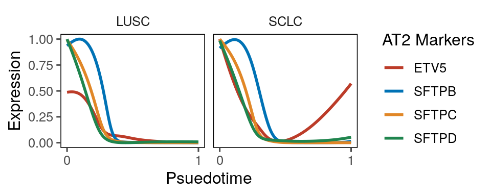
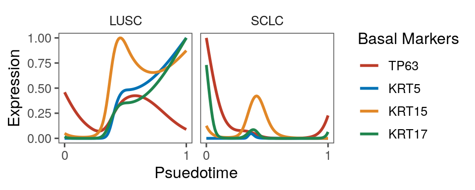
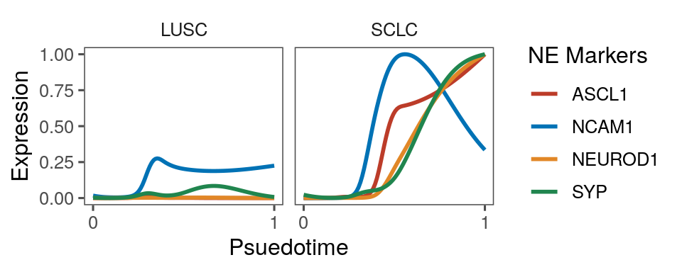
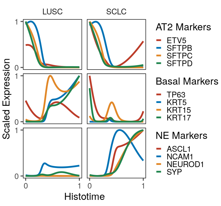
## Figure 5B -- marker expression along the LUSC and SCLC branches
```{r, fig.width = 5, fig.height = 2}
luad_loss_genes <- c("SFTPB", "SFTPC", "SFTPD", "ETV5") #luad loss

p_luad_loss <- ysmooth_df_full %>%
  dplyr::filter(gene %in% luad_loss_genes) %>%
  ggplot(aes(x = time_scaled, y = log_counts_standardized, color = gene, group = gene)) +
  geom_line(linewidth = 1) +
  labs(y = "Expression", color = "AT2 Markers", x = "Psuedotime", linetype = "Lineage") +
  scale_color_nejm() +
  guides(linetype = guide_legend(override.aes = list(linewidth = 1))) +
  scale_x_continuous(breaks = c(0, 1)) +
  theme_few() +
  theme(panel.border = element_rect(fill = NA, color = "black"),
        strip.background = element_blank(),
        axis.line = element_blank()) +
  facet_grid(.~lineage, scales = "free_y")
p_luad_loss
```
```{r, fig.width = 5, fig.height = 2}
lusc_gain_genes <- c("TP63", "KRT5", "KRT15", "KRT17")

p_lusc_gain <- ysmooth_df_full %>%
  dplyr::filter(gene %in% lusc_gain_genes) %>%
  mutate(gene = fct_relevel(gene, lusc_gain_genes)) %>%
  ggplot(aes(x = time_scaled, y = log_counts_standardized, color = gene, group = gene)) +
  geom_line(linewidth = 1) +
  labs(y = "Expression", color = "Basal Markers", x = "Psuedotime", linetype = "Lineage") +
  scale_color_nejm() +
  guides(linetype = guide_legend(override.aes = list(linewidth = 1))) +
  scale_x_continuous(breaks = c(0, 1)) +
  theme_few() +
  facet_grid(.~lineage)
p_lusc_gain
```
```{r, fig.width = 5, fig.height = 2}
sclc_gain_genes <- c("ASCL1", "NCAM1", "NEUROD1", "SYP") # SCLC

p_sclc_gain <- ysmooth_df_full %>%
  dplyr::filter(gene %in% sclc_gain_genes) %>%
  ggplot(aes(x = time_scaled, y = log_counts_standardized, color = gene, group = gene)) +
  geom_line(linewidth = 1) +
  labs(y = "Expression", color = "NE Markers", x = "Psuedotime", linetype = "Lineage") +
  scale_color_nejm() +
  scale_linetype_manual(values = c("solid", "dotted")) +
  guides(linetype = guide_legend(override.aes = list(linewidth = 1))) +
  scale_x_continuous(breaks = c(0, 1)) +
  theme_few() +
  facet_grid(.~lineage)
p_sclc_gain
```
```{r fig5b-histotime-example-genes, fig.width = 3.75, fig.height = 3.5}
pcomb <- (p_luad_loss) + (p_lusc_gain + theme(strip.text.x = element_blank())) + (p_sclc_gain + theme(strip.text.x = element_blank())) + plot_layout(ncol = 1, axes = "collect", axis_titles = "collect") &
  theme(panel.border = element_rect(fill = NA, color = "black"),
        strip.background = element_blank(),
        axis.line = element_blank(), plot.margin = margin(0.8, 0.5, 0.8, 0.5, "mm"),
        legend.margin = margin()) &
  guides(color = guide_legend(keyheight = 0.5, keywidth = 0.5)) &
  scale_y_continuous(breaks = c(0, 1), labels = c(0, 1)) &
  labs(x = "Histotime", y = "Scaled Expression") &
  theme(legend.justification = "left")
ggsave(pcomb, file = here("plots", "histotime_example_genes.pdf"), width = 3.75, height = 3.5)
pcomb
```
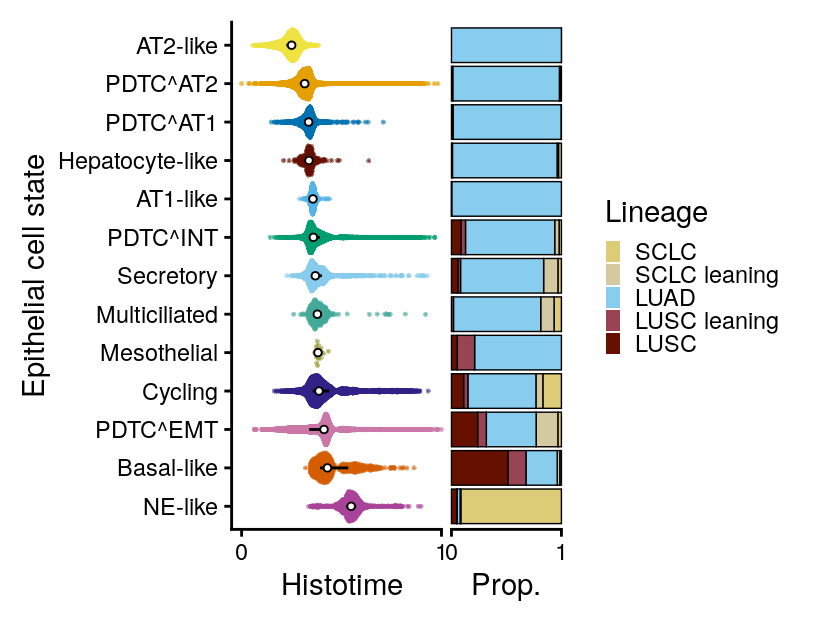
## Figure 5C -- histotime and lineage category by epithelial state
```{r fig5c-histotime-epi-types-dotviolin-wprop, fig.width = 4.25, fig.height = 3.25}
p1 <- srt_ti@meta.data %>%
  ggplot(aes(x = egfrnucseq::standardize(pseudotime), y = fct_reorder(cell_type_epi, -pseudotime, median))) +
  ggrastr::rasterize(geom_quasirandom(aes(color = cell_type_epi), size = 0.1, alpha = 0.5, show.legend = F), dpi = 1000) +
  geom_pointrange(pch = 21,
    stat = "summary", fatten = 2, color = "black", fill = "white", stroke = 0.5,
    fun.min = function(z) {
      quantile(z, 0.25)
    },
    fun.max = function(z) {
      quantile(z, 0.75)
    },
    fun = median, position = position_dodge(width = 0.8)
  ) +
  guides(x = guide_axis(cap = "upper")) +
  scale_color_manual(values = colors$cell_type_epi) +
  scale_x_continuous(breaks = c(0, 1)) +
  labs(x = "Histotime", y = "Epithelial cell state") +
  theme_classic() +
  theme(plot.margin = margin(1,0,1,1, "mm"))

# Distribution over the branches

p2 <- srt_ti@meta.data %>%
  ggplot(aes(y = fct_reorder(cell_type_epi, -pseudotime_scaled, median))) +
  geom_bar(aes(fill = lineage_class_detailed), position = "fill",
           color = "black", linewidth = 0.25) +
  labs(fill = "Lineage", x = "Prop.", y = NULL) +
  scale_x_continuous(expand = c(0,0), breaks = c(0, 1)) +
  guides(x = guide_axis(cap = "both"),
         fill = guide_legend(keywidth = 0.4, keyheight = 0.4, override.aes = list(color = NULL))) +
  scale_fill_manual(values = colors$lineage_class_detailed) +
  theme_classic() +
  theme(axis.text.y = element_blank(),
        axis.line.y = element_blank(),
        axis.ticks.y = element_blank(),
        plot.margin = margin(1,1,1,0, "mm")) +
  coord_cartesian(clip = "off")

pcomb <- p1 + p2 + plot_layout(nrow = 1, widths = c(1, 0.5))
pcomb
ggsave(pcomb, file = here("plots", "histotime_epi_types_dotviolin_wprop.pdf"), width = 4.25, height = 3.25)
```
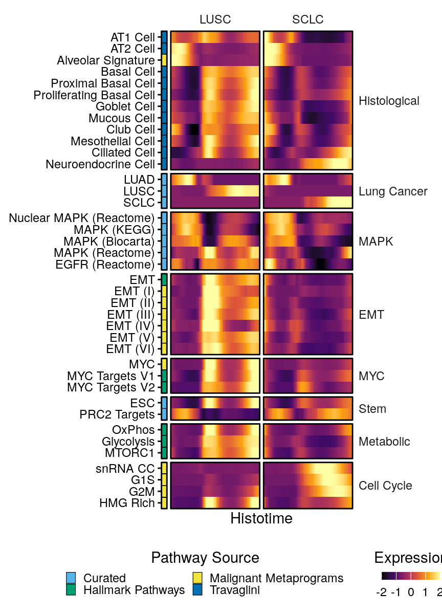
## Figure 5D -- pathway expression within each histotime lineage
Quantify proportions
Load pathways
```{r}
# Use new metaprograms
meta_programs_df <- read.csv(file = here("paper_data", "tirosh_mps_67_natcan_2025.csv"))

meta_programs <- split(meta_programs_df$Gene, meta_programs_df$Geneset)

pathways_v2 <- read.table(here("paper_data", "egfr_pathways_v2.txt"), header = T, sep = "\t")

all_paths <- c(meta_programs, split(pathways_v2$Gene, pathways_v2$pathway))
```
```{r}
library(UCell)
library(BiocParallel)

mat_full <- predictSmooth(models = sce_gam, gene = rownames(sce_gam), nPoints = 100, tidy = FALSE)

ranks <- StoreRankings_UCell(matrix = mat_full, BPPARAM = MulticoreParam(workers = 14, progressbar = T))
histo_scores <- ScoreSignatures_UCell(precalc.ranks = ranks, features = all_paths, name = "", BPPARAM = MulticoreParam(workers = 16, progressbar = T))
```
```{r}
ucell_df <- histo_scores %>%
  as.data.frame() %>%
  rownames_to_column("id") %>%
  separate(id, into = c("lineage_no", "pseudotime_rank")) %>%
  mutate(pseudotime = as.numeric(pseudotime_rank)/100) %>%
  mutate(lineage = factor(lineage_no, levels = c("lineage2", "lineage1"), labels = c("LUSC", "SCLC"))) %>%
  pivot_longer(cols = colnames(histo_scores), names_to = "features.plot", values_to = "Score") %>%
  mutate(features.plot = fct_recode(
    features.plot,
    "LUAD" = "LUAD_GIRARD",
    "LUSC" = "LUSC_GIRARD",
    "SCLC" = "SCLC_CCLE"
  ))
```
```{r}
emt_paths <- grep("emt|HALLMARK_EPITHELIAL_MESENCHYMAL_TRANSITION", ignore.case = T, colnames(histo_scores), value = T)
myc_paths <- c(grep("myc", ignore.case = T, colnames(histo_scores), value = T))
stemness <- c("WONG_EMBRYONIC_STEM_CELL_CORE", "BENPORATH_PRC2_TARGETS")
metabolic_paths <- c("HALLMARK_GLYCOLYSIS", "HALLMARK_OXIDATIVE_PHOSPHORYLATION", "HALLMARK_MTORC1_SIGNALING")
histological_malignant <- c("LUAD", "LUSC", "SCLC")
histological <- c("TRAVAGLINI_LUNG_ALVEOLAR_EPITHELIAL_TYPE_1_CELL", "TRAVAGLINI_LUNG_ALVEOLAR_EPITHELIAL_TYPE_2_CELL", "mp44_alveolar", "TRAVAGLINI_LUNG_BASAL_CELL", "TRAVAGLINI_LUNG_CILIATED_CELL", "TRAVAGLINI_LUNG_CLUB_CELL", "TRAVAGLINI_LUNG_NEUROENDOCRINE_CELL", "TRAVAGLINI_LUNG_PROLIFERATING_BASAL_CELL", "TRAVAGLINI_LUNG_PROXIMAL_BASAL_CELL", "TRAVAGLINI_LUNG_GOBLET_CELL", "TRAVAGLINI_LUNG_MUCOUS_CELL", "TRAVAGLINI_LUNG_MESOTHELIAL_CELL")
cell_cycle <- c(grep("cycle", colnames(histo_scores), ignore.case = T, value = T))
mapk <- c("REACTOME_MAPK_FAMILY_SIGNALING_CASCADES", "REACTOME_MAPK_TARGETS_NUCLEAR_EVENTS_MEDIATED_BY_MAP_KINASES", "BIOCARTA_MAPK_PATHWAY", "KEGG_MAPK_SIGNALING_PATHWAY", "REACTOME_SIGNALING_BY_EGFR")

pth_list <- list(
  "EMT" = emt_paths,
  "MYC" = myc_paths,
  "Stem" = stemness,
  "Metabolic" = metabolic_paths,
  "Lung Cancer" = histological_malignant,
  "Histological" = histological,
  "Cell Cycle" = cell_cycle,
  "MAPK" = mapk
)

pth_cat_df <- enframe(pth_list, name = "Category", value = "features.plot") %>%
  unnest(cols = "features.plot")

pth_df <- ucell_df %>%
  filter(features.plot %in% unlist(pth_list)) %>%
  left_join(pth_cat_df) %>%
  filter(!grepl("_epithelial$", features.plot)) %>%
  filter(!grepl("TGFB", features.plot)) %>%
  mutate(pathway = rename_pathway(features.plot)) %>%
  mutate(
    pathway_source = case_when(
      grepl("^mp", features.plot) ~ "Malignant Metaprograms",
      # grepl("_epithelial$", features.plot) ~ "Epithelial Metaprograms",
      grepl("^TRAVAGLINI", features.plot) ~ "Travaglini",
      grepl("^HALLMARK_", features.plot) ~ "Hallmark Pathways",
      features.plot %in% c("S.Score", "G2M.Score") ~ "Seurat",
      .default = "Curated"
    )
  ) %>%
  # Remove extra myc pathways since they all show the same thing
  filter(
    !(grepl("MYC", features.plot, ignore.case = T) & pathway_source == "Curated")
  ) %>%
  arrange(desc(pathway_source), desc(pathway))
pth_cat_order <- c(
  "Histological", "Lung Cancer", "MAPK", "EMT", "MYC",
  "Stem", "Metabolic", "Cell Cycle"
)

pth_order <- c(
  "G1S", "G2M", "G2M Score", "HMG Rich", "S Score",
  "EMT (I)", "EMT (II)", "EMT (III)", "EMT (IV)", "EMT (V)", "EMT (VI)",
  "LUAD", "LUSC", "SCLC",
  "AT1 Cell", "AT2 Cell", "Alveolar Signature", "Basal Cell", "Proximal Basal Cell",
  "Proliferating Basal Cell", "Goblet Cell", "Mucous Cell", "Club Cell", "Mesothelial Cell", "Ciliated Cell",
  "Neuroendocrine Cell", "MYC", "MYC Targets V1", "MYC Targets V2",
  "Glycolysis", "Oxidative Phosphorylation", "MTORC1", "ESC",
  "PRC2 Targets",
  "Nuclear MAPK (Reactome)", "MAPK (KEGG)", "MAPK (Biocarta)", "MAPK (Reactome)", "EGFR (Reactome)"
)

pth_df <- pth_df %>%
  mutate(
    pathway = fct_relevel(pathway, rev(pth_order)),
    Category = fct_relevel(Category, pth_cat_order)
  )
```
```{r fig5d-histotime-signature-heatmap, fig.height = 6.25, fig.width = 4.5}
p1 <- pth_df %>%
  ggplot(aes(x = "Pathway Source", y = pathway)) +
  geom_tile(aes(fill = pathway_source), color = "black") +
  scale_fill_pander() +
  scale_x_discrete(expand = c(0, 0)) +
  scale_y_discrete(expand = c(0, 0)) +
  theme(
    axis.line.x = element_blank(),
    axis.text.x = element_blank(),
    axis.ticks.x = element_blank(),
    axis.line.y = element_blank(), legend.position = "left", strip.background = element_blank(), strip.text = element_blank()
  ) +
  guides(
    x = guide_axis(angle = 90),
    fill = guide_legend(keywidth = 0.5, keyheight = 0.5, ncol = 2)
  ) +
  facet_grid(Category ~ ., scales = "free", space = "free") +
  labs(y = NULL, x = NULL, fill = "Pathway Source")

p2 <- pth_df %>%
  group_by(pathway) %>%
  mutate(Score_scaled = scale(Score)[,1]) %>%
  ggplot(aes(x = pseudotime, y = pathway)) +
  geom_tile(aes(fill = Score_scaled)) +
  facet_grid(Category~lineage, scales = "free", space = "free") +
  scale_fill_viridis_c(option = "inferno", limits = c(-2, 2), oob = scales::squish) +
  theme(axis.text.x = element_blank(),
        axis.ticks = element_blank(), axis.line = element_blank(),
        strip.background = element_blank(),
        panel.border = element_rect(fill = NA, color = "black"),
        legend.position = "bottom",
        strip.text.y = element_text(hjust = 0, angle = 0)) +
  scale_x_continuous(expand = c(0,0)) +
  scale_y_discrete(expand = c(0,0)) +
  labs(x = "Histotime", y = NULL, fill = "Expression") +
  guides(fill = guide_colorbar(keywidth = 3, keyheight = 0.4))

sig_heatplot <-
  free(
    (p1 +
          theme(plot.margin = margin(l = 0.25, r = 1, unit = "mm"))),
    type = "space", side = "b") +
  free(
    (p2 +
          theme(plot.margin = margin(r = 0.25, unit = "mm"), axis.text.y = element_blank(), axis.ticks.y = element_blank())),
    type = "label", side = "b") +
  plot_layout(guides = "collect", ncol = 2, widths = c(0.03, 1)) +
  plot_annotation(theme = theme(legend.position = "bottom")) &
  theme(panel.spacing = unit(1, "mm"),
        panel.border = element_rect(fill = NA, color = "black", linewidth = 0.5),
        legend.box.margin = margin(), legend.title.position = "top", legend.title = element_text(hjust = 0.5)) &
  coord_cartesian(clip = "off")
ggsave(sig_heatplot, file = here("plots", "histotime_signature_heatmap.pdf"), width = 4.5, height = 6.25)
sig_heatplot
```
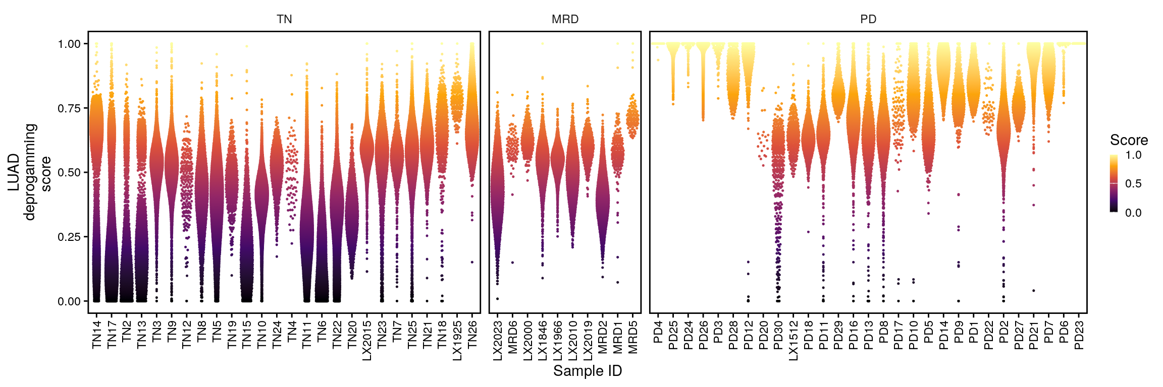
## Figure 5E -- per-specimen histotime summary
If we rescale within the core luad branch we approximate a luad dedifferentiation score?
Perhaps take the 95% percentile as the max clipping.
```{r}
# Winsorised at 0.05/0.99 then standardized upstream, so srt_epi and srt_tum carry
# identical values.
stopifnot(
  "luad_dediff" %in% colnames(srt_ti@meta.data),
  !any(is.na(srt_ti$luad_dediff)),
  all(dplyr::between(srt_ti$luad_dediff, 0, 1))
)
```
Save table with these values
```{r, fig.width = 12, fig.height = 4}
p_linprob_dediff <- srt_ti@meta.data %>%
  arrange(desc(abs(luad_dediff))) %>%
  # filter(lineage_class == "LUAD") %>%
  ggplot(aes(x = fct_reorder(sample_id, (lineage_probability2), mean), y = luad_dediff)) +
  geom_quasirandom(size = 0.01, bandwidth = 3, aes(color = luad_dediff)) +
  guides(
    x = guide_axis(angle = 90),
    color = guide_colorbar(keywidth = 0.4, keyheight = 3)
  ) +
  facet_grid(. ~ time_point, scales = "free", space = "free") +
  scale_color_viridis_c(option = "inferno", breaks = c(0, 0.5, 1)) +
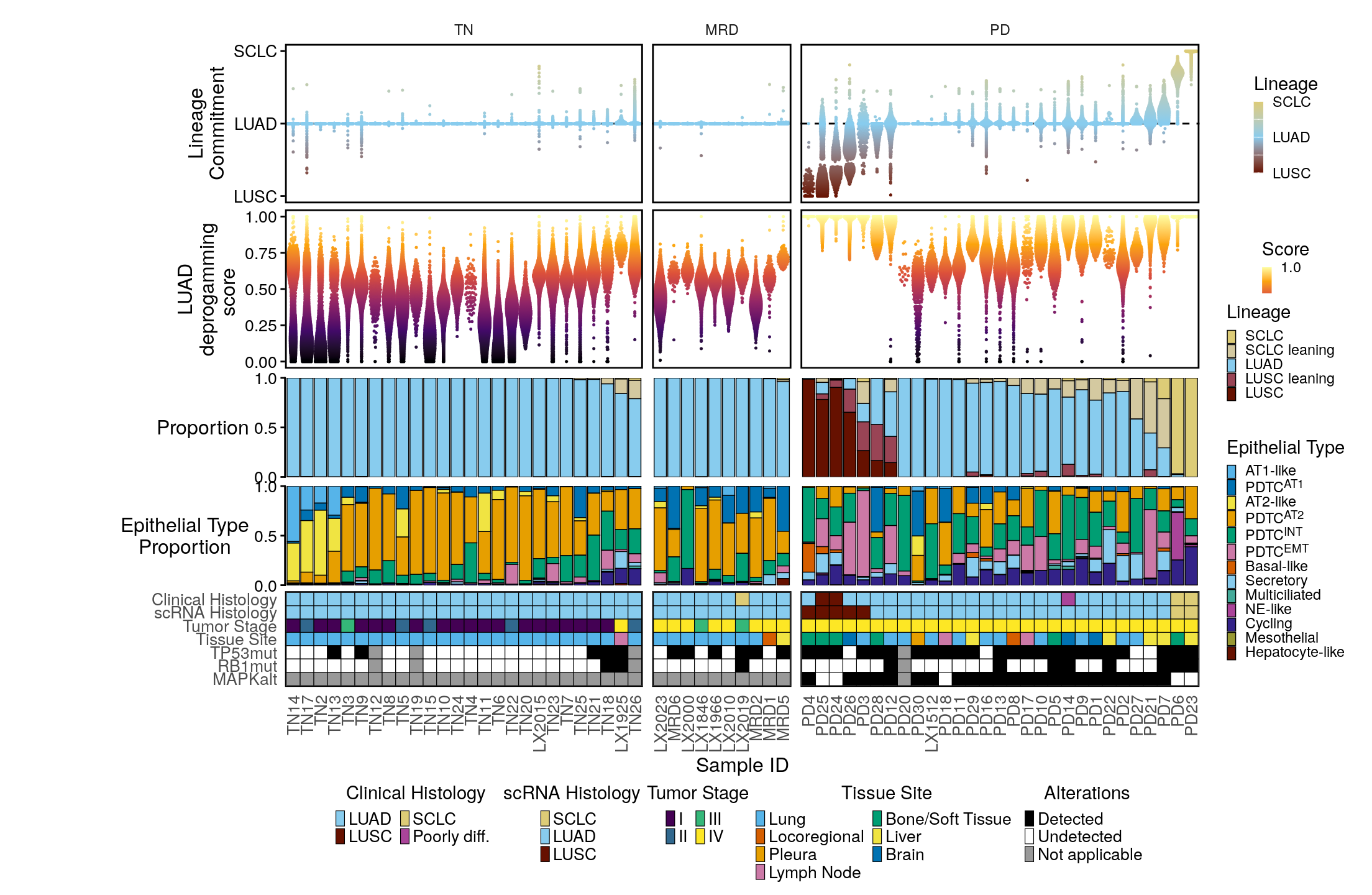
  labs(x = "Sample ID", y = "LUAD\ndeprogamming\nscore ", color = "Score") +
  theme(
    strip.background = element_blank(),
    axis.line = element_blank(),
    panel.border = element_rect(linewidth = 1, fill = NA, color = "black")
  )

p_linprob_dediff <- ggrastr::rasterise(p_linprob_dediff, layers = "Point", dpi = 300)
p_linprob_dediff
```
```{r, fig.width = 9, fig.height = 2.75}
# Of the possibly committed cells how much go each way in each sample
p_linprob_vln <- srt_ti@meta.data %>%
  arrange(desc(abs(lineage_probability2))) %>%
  ggplot(aes(x = fct_reorder(sample_id, (lineage_probability2), mean), y = lineage_probability2)) +
  geom_hline(yintercept = 0, linetype = "dashed", color = "black", alpha = 1) +
  geom_quasirandom(size = 0.01, bandwidth = 2, aes(color = lineage_probability2)) +
  guides(
    x = guide_axis(angle = 90),
    color = guide_colorbar(keywidth = 0.4, keyheight = 3)
  ) +
  facet_grid(. ~ time_point, scales = "free", space = "free") +
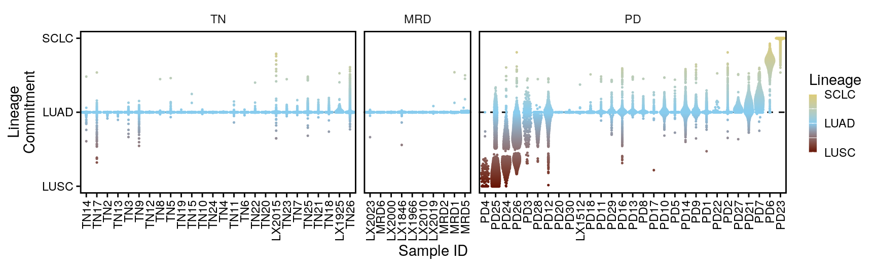
  scale_y_continuous(breaks = c(-1, 0, 1), limits = c(-1, 1), labels = c("LUSC", "LUAD", "SCLC")) +
  scale_color_gradient2(high = colors$histology_predominant_short[["SCLC"]], low = colors$histology_predominant_short[["LUSC"]], mid = colors$histology_predominant_short[["LUAD"]], breaks = c(-1, -0.5, 0, 0.5, 1), limits = c(-1, 1), labels = c("LUSC", "", "LUAD", "", "SCLC")) +
  theme(
    strip.background = element_blank(),
    axis.line = element_blank(),
    panel.border = element_rect(linewidth = 1, fill = NA, color = "black")
  ) +
  labs(x = "Sample ID", y = "Lineage\nCommitment", color = "Lineage")

p_linprob_vln <- ggrastr::rasterise(p_linprob_vln, layers = "Point", dpi = 300)
p_linprob_vln
```
```{r fig5e-lineage-prob-dotviolin-anno, fig.width = 11.5, fig.height = 7.5}
tb_pad <- 0.25

axis_text_size  <- 10
axis_title_size <- 12

library(ggnewscale)

samp_order <- srt_ti@meta.data %>%
  filter(!is.na(lineage_probability2)) %>%
  mutate(sample_id = fct_reorder(sample_id, lineage_probability2, mean)) %>%
  pull(sample_id) %>%
  levels()

anno_df <- srt_ti@meta.data %>%
  filter(!is.na(lineage_probability2)) %>%
  distinct(sample_id, time_point, secondary_mapk, site_of_tissue_simple, histology_predominant_short, scrna_histo, stage_of_tissue_simple, tp53mut, rb1mut, mapk_alt) %>%
  mutate(site_of_tissue_simple = factor(site_of_tissue_simple, levels = names(colors$site_of_tissue_simple)),
         histology_predominant_short = factor(histology_predominant_short, levels = names(colors$histology_predominant_short))) %>%
  mutate(
    across(c(tp53mut, rb1mut), ~ factor(
      ifelse(is.na(.x), "NA", as.character(.x)),
      levels = c("TRUE", "FALSE", "NA")
    )),
    mapk_alt = factor(
      ifelse(is.na(mapk_alt), "NA", as.character(mapk_alt)),
      levels = c("MAPKalt", "Unknown", "NA")
    )
  )

p_anno <- anno_df %>%
  ggplot(aes(x = fct_relevel(sample_id, samp_order))) +
  geom_tile(aes(y = "Clinical Histology", fill = histology_predominant_short), color = "black") +
  scale_fill_manual(
    name = "Clinical Histology", values = colors$histology_predominant_short,
    guide = guide_legend(order = 1, keywidth = 0.4, keyheight = 0.5, ncol = 2, position = "bottom", title.position = "top")
  ) +
  new_scale_fill() +
  geom_tile(aes(y = "scRNA Histology", fill = scrna_histo), color = "black") +
  scale_fill_manual(
    name = "scRNA Histology", values = colors$histology_predominant_short,
    guide = guide_legend(order = 2, keywidth = 0.4, keyheight = 0.5, ncol = 1, position = "bottom", title.position = "top")
  ) +
  new_scale_fill() +
  geom_tile(aes(y = "Tumor Stage", fill = stage_of_tissue_simple), color = "black") +
  scale_fill_viridis_d(
    name = "Tumor Stage",
    guide = guide_legend(order = 3, keywidth = 0.4, keyheight = 0.5, ncol = 2, position = "bottom", title.position = "top")
  ) +
  new_scale_fill() +
  geom_tile(aes(y = "Tissue Site", fill = site_of_tissue_simple), color = "black") +
  scale_fill_manual(
    name = "Tissue Site",
    values = colors$site_of_tissue_simple,
    guide = guide_legend(order = 4, keywidth = 0.4, keyheight = 0.5, ncol = 2, position = "bottom", title.position = "top")
  ) +
  new_scale_fill() +
  geom_tile(aes(y = "TP53mut", fill = tp53mut), color = "black") +
  scale_fill_manual(
    name = "Alterations",
    values = c("TRUE" = "black", "FALSE" = "white", "NA" = "grey60"), breaks = c("TRUE", "FALSE", "NA"),
    labels = c("Detected", "Undetected", "Not applicable"),

    drop = FALSE,
    guide = guide_legend(order = 5, keywidth = 0.4, keyheight = 0.1, ncol = 1, position = "bottom", title.position = "top")
  ) +
  new_scale_fill() +
  geom_tile(aes(y = "RB1mut", fill = rb1mut), color = "black", show.legend = F) +
  scale_fill_manual(
    values = c("TRUE" = "black", "FALSE" = "white", "NA" = "grey60"), breaks = c("TRUE", "FALSE", "NA"),
    labels = c("Detected", "Undetected", "Not applicable"),
    drop = FALSE,
    guide = "none"
  ) +
  new_scale_fill() +
  geom_tile(aes(y = "MAPKalt", fill = mapk_alt), color = "black", show.legend = F) +
  scale_fill_manual(
    values = c("MAPKalt" = "black", "Unknown" = "white", "NA" = "grey60"),
    breaks = c("MAPKalt", "Unknown", "NA"),
    labels = c("Detected", "Undetected", "Not applicable"),
    drop = FALSE,
    guide = "none"
  ) +
  facet_grid(. ~ time_point, scales = "free", space = "free") +
  theme_minimal() +
  theme(panel.background = element_blank(), panel.grid = element_blank()) +
  theme(
    strip.text = element_blank(),
    legend.title = element_text(hjust = 0.5),
    legend.text = element_text(size = 10, margin = margin(l = 2, r = 4)),
    legend.key.spacing.x = unit(1, "pt"),
    legend.key.spacing.y = unit(1, "pt"),
    legend.spacing.x = unit(4, "pt"),
    legend.margin = margin(0, 0, 0, 0),
    legend.box.spacing = unit(4, "pt")
  ) +
  labs(fill = "Tissue Site", y = NULL) +
  scale_y_discrete(limits = rev(c(
    "Clinical Histology",
    "scRNA Histology",
    "Tumor Stage",
    "Tissue Site",
    "TP53mut",
    "RB1mut",
    "MAPKalt"
  ))) +
    guides(x = guide_axis(angle = 90))

p_prop_combined <- srt_ti@meta.data %>%
  filter(!is.na(lineage_probability2)) %>%
  ggplot(aes(x = fct_relevel(sample_id, samp_order))) +
  geom_bar(aes(fill = lineage_class_detailed), position = "fill",
           color = "black", linewidth = 0.25) +
  facet_grid(. ~ time_point, scales = "free", space = "free") +
  scale_fill_manual(values = colors$lineage_class_detailed) +
  guides(
    x = guide_axis(angle = 90),
    y = guide_axis(cap = "both"),
    fill = guide_legend(keywidth = 0.4, keyheight = 0.4)
  ) +
  labs(y = "Proportion", x = NULL, fill = "Lineage") +
  scale_y_continuous(expand = c(0, 0)) +
  theme(
    strip.text = element_blank(),
    axis.text.x = element_blank(),
    axis.line.x = element_blank(),
    axis.ticks.x = element_blank(),
    axis.title.y = element_text(angle = 0, vjust = 0.5)
  ) +
  scale_y_continuous(breaks = c(0, 0.5, 1))

p_branch_prop <- srt_ti@meta.data %>%
  filter(!is.na(lineage_probability2)) %>%
  ggplot(aes(x = fct_relevel(sample_id, samp_order))) +
  geom_bar(aes(fill = fct_relevel(lineage_class, names(colors$histology_predominant_short))), position = "fill") +
  facet_grid(. ~ time_point, scales = "free", space = "free") +
  scale_fill_manual(values = colors$histology_predominant_short) +
  guides(
    x = guide_axis(angle = 90),
    y = guide_axis(cap = "both"),
    fill = guide_legend(keywidth = 0.4, keyheight = 0.4)
  ) +
  labs(y = "Proportion\n(In branch)", x = NULL, fill = "Lineage") +
  scale_y_continuous(expand = c(0, 0)) +
  theme(
    strip.text = element_blank(),
    axis.text.x = element_blank(),
    axis.line.x = element_blank(),
    axis.ticks.x = element_blank(),
    axis.title.y = element_text(angle = 0, vjust = 0.5)
  ) +
  scale_y_continuous(breaks = c(0, 0.5, 1))

p_epi_type_prop <- srt_ti@meta.data %>%
  filter(!is.na(lineage_probability2)) %>%
  ggplot(aes(x = fct_relevel(sample_id, samp_order))) +
  geom_bar(aes(fill = cell_type_epi), position = "fill",
           color = "black", linewidth = 0.25) +
  facet_grid(. ~ time_point, scales = "free", space = "free") +
  scale_fill_manual(values = colors$cell_type_epi, labels = label_md) +
  guides(
    x = guide_axis(angle = 90),
    y = guide_axis(cap = "both"),
    fill = guide_legend(keywidth = 0.4, keyheight = 0.4)
  ) +
  labs(y = "Epithelial Type\nProportion", x = NULL, fill = "Epithelial Type")

p_prop <-
  free(p_prop_combined, type = "label", side = "l") +
  free(p_epi_type_prop, type = "label", side = "l") +
  plot_layout(ncol = 1, guides = "collect") &
  theme(
    strip.text = element_blank(),
    axis.text.x = element_blank(),
    axis.line.x = element_blank(),
    axis.ticks.x = element_blank(),
    axis.title.y = element_text(angle = 0, vjust = 0.5),
    legend.text = ggtext::element_markdown()
  ) &
  scale_y_continuous(expand = c(0, 0), breaks = c(0, 0.5, 1))

pcomb <-
  free((p_linprob_vln + labs(x = NULL) + theme(axis.text.x = element_blank(), axis.ticks.x = element_blank(), plot.margin = margin(t = tb_pad, b = 0, unit = "lines"))), type = "label", side = "l") +
  free((p_linprob_dediff + labs(x = NULL) + theme(strip.text = element_blank(), strip.background = element_blank(), axis.lines = element_blank(), strip.clip = "off", panel.border = element_rect(fill = NA), axis.text.x = element_blank(), axis.ticks.x = element_blank(), plot.margin = margin(t = tb_pad, b = 0, unit = "lines"))), type = "label", side = "l") +
  free((p_prop + theme(plot.margin = margin())), type = "label", side = "l") + (p_anno + labs(x = "Sample ID") + theme(plot.margin = margin(t = tb_pad, b = tb_pad, unit = "lines")) + guides(x = guide_axis(angle = 90))) + plot_layout(ncol = 1, heights = c(1, 1, 1.3, 0.6)) &
  theme(
    axis.text  = element_text(size = axis_text_size),
    axis.title = element_text(size = axis_title_size),
    panel.background = element_rect(fill = "white")

  )
pcomb
ggsave(pcomb, file = here("plots", "lineage_prob_dotviolin_anno.pdf"), width = 11.5, height = 7.5)
```
# Figure S10 -- Histotime analysis
## Figure S10A -- TF regulon activity over the histotime branches
```{r}
pred_curves <- readRDS(here("paper_data", "beta_gam_tf_pred_curves.rds"))
endpoint_de <- readRDS(here("paper_data", "beta_gam_tf_de_tests.rds"))$endpoint

pred_curves <- pred_curves %>%
  mutate(lineage = factor(lineage, levels = c(2,1), labels = c("LUSC", "SCLC"))) %>%
  group_by(lineage) %>%
  mutate(histotime = standardize(pseudotime))

# Annotated bifurcation point
bif_pt <- quantile(srt_ti@meta.data[srt_ti$lineage_class == "LUAD",]$pseudotime_scaled, prob = c(0.99))
```
The TF regulons that are also differentially expressed at the trajectory endpoints.
```{r}
tf_list <- intersect(endpoint_de$feature, ysmooth_df_full$gene)
```
```{r}
mat <- pred_curves %>%
  group_by(lineage, feature) %>%
  mutate(step = rank(histotime)) %>%
  filter(feature %in% tf_list) %>%
  pivot_wider(id_cols = "feature", names_from = c("lineage", "step"), values_from = "fit") %>%
  column_to_rownames("feature") %>%
  as.matrix()
mat_scaled <- scale(mat)

dmat <- 1 - coop::cosine(t(mat_scaled))
dmat <- as.dist(dmat)

nn <- FindNeighbors(dmat, annoy.metric = "cosine", k.param = 10, nn.method = "annoy")

cluster <- scatools::leiden_wrapper(nn$snn, resolution = 1, group_singletons = T)
cls_df <- data.frame(gene = names(cluster), cluster = cluster)
```
```{r}
# Classify TFs into four trajectory patterns using peak histotime heuristics
early_thresh <- bif_pt
late_thresh  <- 0.7

pattern_df <- pred_curves %>%
  inner_join(cls_df, by = c("feature" = "gene")) %>%
  group_by(feature) %>%
  mutate(fit_scale = scale(fit)[,1],
         std_exp = standardize(fit_scale))

# Per-gene peak histotime and scaled expression at peak in each lineage
peak_by_lineage <- pattern_df %>%
  group_by(feature, lineage) %>%
  summarise(
    peak_time = histotime[which.max(fit_scale)],
    peak_val  = max(fit_scale),
    .groups = "drop"
  ) %>%
  pivot_wider(names_from = lineage,
              values_from = c(peak_time, peak_val),
              names_sep = "_")

peak_by_lineage <- peak_by_lineage %>%
  mutate(peak_val_diff = peak_val_LUSC - peak_val_SCLC)  # positive = stronger in LUSC

peak_by_lineage <- peak_by_lineage %>%
  mutate(tf_pattern = case_when(
    # Both peak early → losing LUAD identity
    peak_time_LUSC <= early_thresh & peak_time_SCLC <= early_thresh ~ "LUAD deprogramming",
    # Late peak with expression bias
    peak_time_LUSC >= late_thresh & peak_val_diff >= 0.5 ~ "LUSC commitment",
    peak_time_SCLC >= late_thresh & peak_val_diff <= -0.5 ~ "SCLC commitment",
    # Both peak late but balanced
    peak_time_LUSC >= late_thresh & peak_time_SCLC >= late_thresh ~ "Shared late",
    # Intermediate peak with expression bias → leaning toward one lineage
    peak_val_diff >= 0.5 & peak_time_LUSC >= early_thresh  ~ "LUSC early",
    peak_val_diff <= -0.5 & peak_time_SCLC >= early_thresh ~ "SCLC early",
    # Intermediate peak, balanced expression
    peak_time_LUSC < late_thresh & peak_time_LUSC > early_thresh & peak_time_SCLC < late_thresh & peak_time_SCLC > early_thresh ~ "Shared transitional",
    TRUE ~ "Other"
  ))

# Order: LUAD deprogramming first, then shared, then leaning, then committed
pattern_levels <- c("LUAD deprogramming", "Shared transitional",
                    "LUSC early", "LUSC commitment",
                    "SCLC early", "SCLC commitment",
                    "Shared late", "Other")
peak_by_lineage$tf_pattern <- factor(peak_by_lineage$tf_pattern, levels = pattern_levels)

pattern_df <- pattern_df %>%
  left_join(peak_by_lineage %>% dplyr::select(feature, peak_time_LUSC, peak_time_SCLC,
                                        peak_val_LUSC, peak_val_SCLC,
                                        peak_val_diff, tf_pattern),
            by = "feature")

# Group the LUSC and SCLC patterns
pattern_df$tf_pattern_coarse <- case_when(
  pattern_df$tf_pattern %in% c("LUSC early", "LUSC commitment") ~ "LUSC-associated",
  pattern_df$tf_pattern %in% c("SCLC early", "SCLC commitment") ~ "SCLC-associated",
  pattern_df$tf_pattern %in% c("Shared late", "Other") ~ "Other",
  TRUE ~ pattern_df$tf_pattern
)
pattern_df$tf_pattern_coarse <- factor(pattern_df$tf_pattern_coarse, levels = c("LUAD deprogramming", "Shared transitional",
                                            "LUSC-associated", "SCLC-associated", "Other"))
```
```{r}
markers_select <- list(
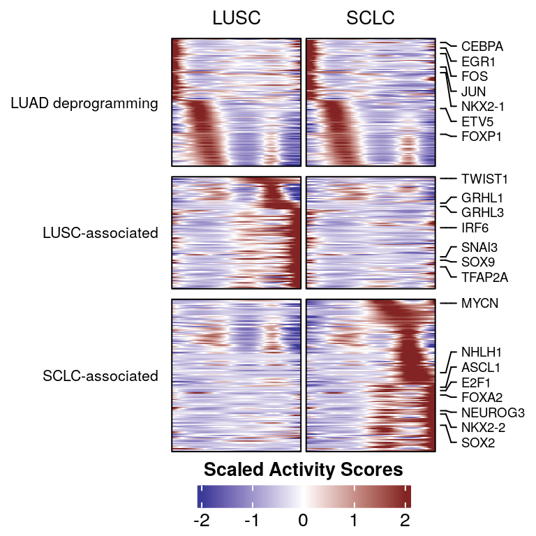
  `LUAD deprogramming` = c("NKX2-1", "ETV5", "CEBPA", "FOXP1", "FOS", "EGR1", "JUN"),
  `LUSC-associated`    = c("GRHL3", "GRHL1", "IRF6", "SOX9", "TFAP2A", "TWIST1", "SNAI3"),
  `SCLC-associated`    = c("ASCL1", "NKX2-2", "NEUROG3", "NHLH1", "SOX2", "FOXA2", "MYCN", "E2F1")
)
```
```{r}
# ggrepel is attached here for the S10E scatter labels further down.
library(ggrepel)

# Row order for the heatmap: within each pattern, by overall peak histotime.
g_ord <- pattern_df %>%
  group_by(feature) %>%
  summarise(peak_time = histotime[which.max(fit_scale)]) %>%
  arrange(desc(peak_time), desc(feature)) %>%
  pull(feature)
```
```{r figs10a-lineage-histotime-tf-peak-patterns-focus-ch, fig.width = 4, fig.height = 4}
library(ComplexHeatmap)
library(circlize)

# Build matrix: rows = genes, cols = histotime steps within each lineage
heat_df <- pattern_df %>%
  filter(tf_pattern_coarse != "Other") %>%
  group_by(feature, lineage) %>%
  mutate(step = row_number()) %>%
  ungroup()

heat_mat <- heat_df %>%
  pivot_wider(id_cols = "feature", names_from = c("lineage", "step"), values_from = "fit_scale") %>%
  column_to_rownames("feature") %>%
  as.matrix()

heat_mat <- heat_mat[rev(g_ord[g_ord %in% rownames(heat_mat)]), ]

# Row split by tf_pattern_coarse
row_pattern <- pattern_df %>%
  filter(tf_pattern_coarse != "Other") %>%
  distinct(feature, tf_pattern_coarse) %>%
  deframe()
row_split <- factor(row_pattern[rownames(heat_mat)],
                    levels = c("LUAD deprogramming", "LUSC-associated", "SCLC-associated"))

# Column split by lineage
n_steps <- heat_df %>% distinct(lineage, step) %>% dplyr::count(lineage) %>% pull(n) %>% unique()
col_split <- rep(c("LUSC", "SCLC"), each = n_steps)

# anno_mark for selected genes
mark_genes <- unlist(markers_select)
mark_idx <- which(rownames(heat_mat) %in% mark_genes)
mark_labels <- rownames(heat_mat)[mark_idx]

row_anno <- rowAnnotation(
  marks = anno_mark(
    at = mark_idx,
    labels = mark_labels,
    labels_gp = gpar(fontsize = 7),
    link_width = unit(4, "mm")
  )
)

col_fun <- colorRamp2(c(-2, 0, 2), c(scales::muted("blue"), "white", scales::muted("red")))

ht <- Heatmap(
  heat_mat,
  name = "Scaled\nActivity",
  col = col_fun,
  row_split = row_split,
  column_split = rev(col_split),
  cluster_rows = FALSE,
  cluster_columns = FALSE,
  show_row_names = FALSE,
  show_column_names = FALSE,
  row_title_rot = 0,
  row_title_gp = gpar(fontsize = 8),
  column_title_gp = gpar(fontsize = 10),
  row_gap = unit(2, "mm"),
  column_gap = unit(1, "mm"),
  border = TRUE,
  right_annotation = row_anno,
  heatmap_legend_param = list(
    title = "Scaled Activity Scores",
    legend_width = unit(4, "cm"),
    legend_title_gp = gpar(fontsize = 10),
    title_position = "topcenter",
    direction = "horizontal"
  ),
  column_title = c("LUSC", "SCLC")
)

pdf(here("plots", "lineage_histotime_tf_peak_patterns_focus_ch.pdf"), width = 4, height = 4)
draw(ht, heatmap_legend_side = "bottom", merge_legend = TRUE)
dev.off()
draw(ht, heatmap_legend_side = "bottom", merge_legend = TRUE)
```
## Figure S10B -- LUAD deprogramming in MAPKalt vs MAPKnd PD
```{r figs10b-mapkalt-pd-luad-dediff, fig.width = 1.75, fig.height = 2}
p <- srt_ti@meta.data %>%
  filter(time_point == "PD" & mapk_alt != "NA") %>%
  ggplot(aes(x = fct_rev(mapk_alt), y = luad_dediff)) +
  geom_violin(scale = "width", aes(fill = mapk_alt), show.legend = F) +
  scale_fill_aaas() +
  geom_boxplot(width = 0.2, outliers = F) +
  scale_y_continuous(breaks = c(0, 0.5, 1)) +
  guides(y = guide_axis(cap = "both"),
         x = guide_axis(cap = "both")) +
  ggpubr::geom_pwc(label = "p.signif", tip.length = 0, vjust = 0.5) +
  coord_cartesian(clip = "off") +
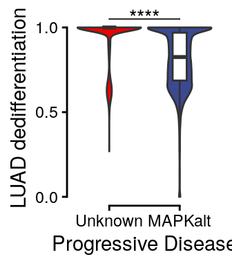
  labs(x = "Progressive Disease", y = "LUAD dedifferentiation")
p
ggsave(p, file = here("plots", "MAPKalt_PD_luad_dediff.pdf"), width = 1.75, height = 2)
```
## Figure S10C-D -- panel-independent 30-NN validation of lineage priming
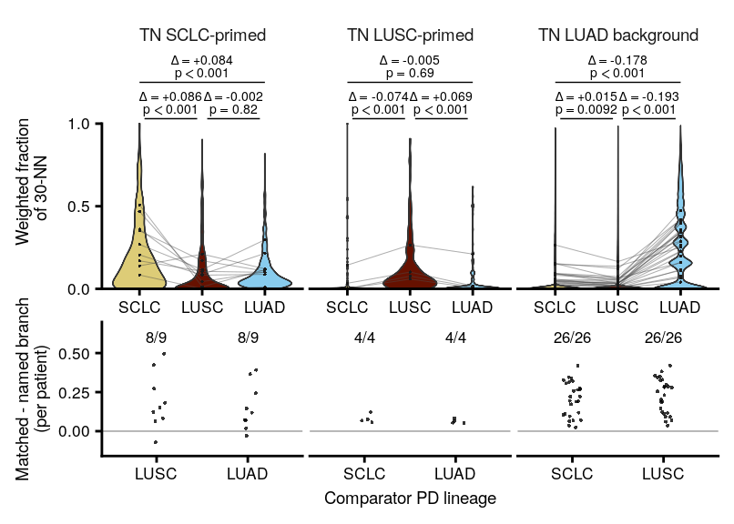
For every treatment-naive cell we take its 30 nearest neighbours there and measure what fraction fall in each progression branch.
```{r figs10cd-constants}
library(BiocNeighbors)

# Seeded separately from the notebook-wide seed: the deposited Annoy run was
# produced at 3, and the recompute path has to match it.
set.seed(3)

K        <- 30                                     # neighbours per cell
DIMS     <- 1:30                                   # latent dimensions the k-NN runs in
BRANCHES <- c("pd_sclc", "pd_lusc", "pd_luad")

# The batch-corrected epithelial manifold -- the space cell_type_epi was defined on.
# 00_download_convert.qmd lower-cases reduction names.
EMBEDDING <- "rnasoup_rpca_integrated"

# Figures say "lineage-primed"; the `tn_class` levels stay "...-leaning" so the code keys
# match the analysis repo. `primed_lab()` maps one to the other at plotting time.
PRIMED_LABS <- c("TN SCLC-leaning"    = "TN SCLC-primed",
                 "TN LUSC-leaning"    = "TN LUSC-primed",
                 "TN LUAD background" = "TN LUAD background")
primed_lab <- function(x) unname(PRIMED_LABS[as.character(x)])
```
```{r figs10cd-assert-definition}
stopifnot(all(c("Histotime_s", "lineage_probability", "lineage_probability2",
                "lineage_class_coarse") %in% colnames(srt_ti@meta.data)))
stopifnot(isTRUE(all.equal(srt_ti$lineage_probability2,
                           srt_ti$lineage_probability * srt_ti$Histotime_s)))

coarse_chk <- dplyr::case_when(
  srt_ti$lineage_probability2 >=  0.05 ~ "SCLC",
  srt_ti$lineage_probability2 <= -0.05 ~ "LUSC",
  .default = "LUAD"
)
stopifnot(identical(coarse_chk, as.character(srt_ti$lineage_class_coarse)))
```
The panel PCA is deposited as `histotime` and must never be the embedding used here --
the independence argument rests on that.
```{r figs10cd-assert-bindings}
srt_ti$patient <- as.character(srt_ti$patient)

stopifnot(
  all(c("lineage_class_coarse", "time_point", "sample_id", "patient",
        "cell_id", "is_tumor_cell") %in% colnames(srt_ti@meta.data)),
  EMBEDDING %in% Reductions(srt_ti),
  ncol(Embeddings(srt_ti, EMBEDDING)) >= max(DIMS),
  !EMBEDDING %in% c("pca_genes", "histotime"),
  all(srt_ti$cell_type == "Tumor Cell"),
  all(srt_ti$is_tumor_cell)
)

stopifnot(
  dplyr::n_distinct(srt_ti$patient) == dplyr::n_distinct(srt_ti$sample_id),
  dplyr::n_distinct(paste(srt_ti$patient, srt_ti$sample_id)) ==
    dplyr::n_distinct(srt_ti$patient)
)

cli::cli_alert_success("Bindings verified: {ncol(srt_ti)} tumor cells")
```
```{r figs10cd-panel-overlap}
panel_genes <- readxl::read_excel(here("paper_data", "supplemental_tables.xlsx"),
                                  sheet = "Table S7 - Histotime Features")$Gene %>%
  unique()
stopifnot(length(panel_genes) == 179)
```
```{r figs10cd-cell-sets}
md_raw <- srt_ti@meta.data

stopifnot(identical(as.character(md_raw$cell_id), rownames(md_raw)))
md_raw$cell_id <- rownames(md_raw)

md <- md_raw %>%
  dplyr::select(cell_id, sample_id, patient, time_point, lineage_class_coarse) %>%
  filter(time_point %in% c("TN", "PD")) %>%
  mutate(
    time_point = factor(time_point, levels = c("TN", "PD")),
    grp = factor(paste(time_point, lineage_class_coarse, sep = "_"),
                 levels = c("TN_SCLC", "TN_LUAD", "TN_LUSC",
                            "PD_SCLC", "PD_LUAD", "PD_LUSC")),
    tn_class = case_when(
      time_point == "TN" & lineage_class_coarse == "SCLC" ~ "TN SCLC-leaning",
      time_point == "TN" & lineage_class_coarse == "LUSC" ~ "TN LUSC-leaning",
      time_point == "TN" & lineage_class_coarse == "LUAD" ~ "TN LUAD background",
      TRUE ~ NA_character_
    ) %>% factor(levels = c("TN SCLC-leaning", "TN LUSC-leaning", "TN LUAD background"))
  )

stopifnot(!any(is.na(md$grp)))
```
Each neighbour is weighted by the inverse size of its identity group, so the metric is
not driven by population size.
```{r figs10cd-helpers}
# Inverse-frequency-weighted neighbour composition. nn_idx holds reference-local
# indices; returns an [n_query x n_levels] matrix whose rows sum to 1.
neighbor_frac_weighted <- function(nn_idx, ref_group) {
  ref_group <- as.factor(ref_group)
  stopifnot(max(nn_idx) <= length(ref_group), min(nn_idx) >= 1)

  # w_j = 1 / n_{group(j)}, exactly as calc_snn_specificity
  w <- as.numeric((1 / table(ref_group))[as.character(ref_group)])

  nb_w   <- matrix(w[nn_idx], nrow = nrow(nn_idx))                 # weight of each neighbour
  nb_grp <- matrix(as.integer(ref_group)[nn_idx], nrow = nrow(nn_idx))

  denom <- rowSums(nb_w)
  out <- vapply(seq_along(levels(ref_group)), function(g) {
    rowSums(nb_w * (nb_grp == g)) / denom
  }, numeric(nrow(nn_idx)))

  colnames(out) <- levels(ref_group)
  out
}

# k-NN from a reference set to a query set, dropping self-matches. Returns
# reference-local indices, so the result indexes ref_group directly.
query_knn <- function(emb, query_idx, ref_idx, k) {
  X <- emb[ref_idx, , drop = FALSE]
  Q <- emb[query_idx, , drop = FALSE]

  # request k+1 so a dropped self-match does not cost us a neighbour
  res <- BiocNeighbors::queryKNN(X = X, query = Q, k = k + 1, BNPARAM = AnnoyParam())
  loc <- res$index                                    # reference-local already

  # a self-match is a local index whose global id equals the query's own global id
  self <- matrix(ref_idx[loc], nrow = nrow(loc)) ==
    matrix(query_idx, nrow = length(query_idx), ncol = ncol(loc))

  out <- t(vapply(seq_len(nrow(loc)), function(i) {
    keep <- loc[i, ][!self[i, ]]
    keep[seq_len(k)]
  }, numeric(k)))

  storage.mode(out) <- "integer"
  stopifnot(!anyNA(out))
  out
}
```
Query = TN cells. Reference = all TN + PD tumour cells. For each TN cell, the weighted
fraction of its `K` nearest neighbours falling in each PD branch.
`AnnoyParam()` is approximate, so the figure is reproduced from the deposited run in
`paper_data/pd_neighbor_fractions.txt.gz` rather than by repeating the search. Set
`RECOMPUTE <- TRUE` to run it instead.
```{r figs10cd-neighbor-fractions}
RECOMPUTE <- FALSE

if (RECOMPUTE) {
  ref_idx   <- seq_len(nrow(md))                      # all TN + PD cells
  query_idx <- which(md$time_point == "TN")

  emb <- Embeddings(srt_ti, EMBEDDING)[md$cell_id, DIMS]

  cli::cli_alert_info("k-NN over {length(query_idx)} TN cells, k = {K}")
  nn <- query_knn(emb, query_idx, ref_idx, K)
  fr <- neighbor_frac_weighted(nn, md$grp[ref_idx])

  res <- tibble(
    cell_id = md$cell_id[query_idx],
    pd_sclc = fr[, "PD_SCLC"],
    pd_lusc = fr[, "PD_LUSC"],
    pd_luad = fr[, "PD_LUAD"]
  ) %>%
    left_join(md %>% dplyr::select(cell_id, sample_id, patient, tn_class), by = "cell_id")
} else {
  res <- read.table(here("paper_data", "pd_neighbor_fractions.txt.gz"),
                    header = TRUE, sep = "\t")
}

stopifnot(dplyr::setequal(res$cell_id, md$cell_id[md$time_point == "TN"]),
          !anyDuplicated(res$cell_id),
          all(BRANCHES %in% colnames(res)))

res <- res %>%
  mutate(tn_class = factor(tn_class, levels = c("TN SCLC-leaning", "TN LUSC-leaning",
                                                "TN LUAD background")))
```
Brackets on the upper row are a two-sided *t* on the per-cell branch difference with
standard errors clustered by patient (df = G - 1). Every pairwise comparison is drawn,
significant or not, with the effect size alongside the p.
The lower row plots, for each patient with at least `MIN_CELLS` cells of a class, that
patient's own matched-minus-named-branch difference; the k/n labels count how many fall
above zero.
```{r figs10cd-figure-stats}
# A patient needs enough cells for its mean to mean anything; the number clearing this bar in
# each class is printed below.
MIN_CELLS <- 10

branch_short <- c(pd_sclc = "PD-SCLC", pd_lusc = "PD-LUSC", pd_luad = "PD-LUAD")
branch_fills <- c(pd_sclc = "#DDCC77", pd_lusc = "#661100", pd_luad = "#88CCEE")

# The branch each TN class is supposed to sit nearest. For background that is PD-LUAD, which
# makes the control panel a positive result rather than an empty slot.
matched_branch_all <- c("TN SCLC-leaning"    = "pd_sclc",
                        "TN LUSC-leaning"    = "pd_lusc",
                        "TN LUAD background" = "pd_luad")

df_alt <- res %>%
  dplyr::select(cell_id, patient, tn_class, all_of(BRANCHES)) %>%
  pivot_longer(all_of(BRANCHES), names_to = "branch", values_to = "frac") %>%
  mutate(branch = factor(branch, levels = BRANCHES))

# Per patient, per class: the mean fraction in each branch, and which one is the matched branch.
pat_wide <- res %>%
  group_by(tn_class, patient) %>%
  summarise(n_cells = n(), across(all_of(BRANCHES), mean), .groups = "drop") %>%
  filter(n_cells >= MIN_CELLS) %>%
  mutate(matched = case_when(tn_class == "TN SCLC-leaning" ~ pd_sclc,
                             tn_class == "TN LUSC-leaning" ~ pd_lusc,
                             TRUE                          ~ pd_luad))

pat_alt <- pat_wide %>%
  pivot_longer(all_of(BRANCHES), names_to = "branch", values_to = "frac") %>%
  mutate(branch = factor(branch, levels = BRANCHES),
         is_matched = as.character(branch) == matched_branch_all[as.character(tn_class)])

# Per-patient difference: matched minus each of the two other branches. Levels follow branch
# order so the mismatched contrast always precedes the PD-LUAD one, matching the bracket order.
delta_alt <- pat_alt %>%
  filter(!is_matched) %>%
  mutate(delta = matched - frac,
         contrast = factor(paste("vs", branch_short[as.character(branch)]),
                           levels = paste("vs", branch_short[BRANCHES])))

n_up_alt <- delta_alt %>%
  group_by(tn_class, contrast) %>%
  summarise(lab = glue("{sum(delta > 0)}/{n()}"), .groups = "drop")

# Two-sided t on the per-cell branch difference, SEs clustered by patient. Survives the
# few-evaluable-patient LUSC problem that floors a signed-rank test.
cluster_t <- function(x, g) {
  n <- length(x); G <- dplyr::n_distinct(g); m <- mean(x)
  Sg <- vapply(split(x - m, g), sum, numeric(1))     # residual sum within each patient
  se <- sqrt(sum(Sg^2) / n^2 * (G / (G - 1)))
  2 * pt(-abs(m / se), df = G - 1)                   # t(G-1): conservative for few clusters
}

# Adjacent pairs share the lower rung, the spanning pair sits above; the lower two are inset by
# GAP so they do not read as one line.
GAP <- 0.08

BRACKET_PAIRS <- tribble(
  ~a,         ~b,         ~x,       ~xend,    ~y,
  "pd_sclc",  "pd_lusc",   1 + GAP,  2 - GAP, 1.03,
  "pd_lusc",  "pd_luad",   2 + GAP,  3 - GAP, 1.03,
  "pd_sclc",  "pd_luad",   1,        3,       1.25
)

brackets <- expand_grid(tn_class = levels(res$tn_class), BRACKET_PAIRS) %>%
  pmap_dfr(function(tn_class, a, b, x, xend, y) {
    d <- res %>% filter(tn_class == !!tn_class)
    tibble(tn_class = tn_class, a = a, b = b, x = x, xend = xend, y = y,
           mean_diff = mean(d[[a]] - d[[b]]),
           p         = cluster_t(d[[a]] - d[[b]], d$patient))
  }) %>%
  mutate(tn_class = factor(tn_class, levels = levels(res$tn_class)),
         # Two single-line plotmath layers rather than one atop(), which would detach the pair
         # from its bracket. parse = TRUE draws the delta through the symbol font (unicode tofus).
         lab_delta = glue('Delta == "{sprintf("%+.3f", mean_diff)}"'),
         lab_p     = dplyr::if_else(p < 0.001, "p < 0.001", glue("p == {signif(p, 2)}")))
theme_alt <- theme(strip.background = element_blank(),
                   strip.text       = element_text(size = 7),
                   axis.text        = element_text(size = 6.5),
                   axis.title.y     = element_text(size = 7),
                   panel.grid.minor = element_blank(),
                   panel.spacing    = unit(3, "pt"),
                   plot.margin      = margin(1, 1, 1, 1))
```
```{r figs10cd-pd-neighbor-fraction-lineage-matched-transposed, fig.width = 4.2, fig.height = 3.0}
# --- Figure S10C: weighted 30-NN fraction by PD branch, faceted by TN class ---
alt_top <- df_alt %>%
  ggplot(aes(branch, frac)) +
  ggrastr::rasterize(
    geom_violin(aes(fill = branch), scale = "width", width = 0.85, linewidth = 0.25,
                quantiles = 0.5),
    dpi = 600
  ) +
  # One line per patient: replication is visible directly, without singling any patient out.
  geom_line(data = pat_alt, aes(group = patient), colour = "grey30", linewidth = 0.18, alpha = 0.45) +
  geom_point(data = pat_alt, colour = "grey10", size = 0.6, stroke = 0) +
  geom_segment(data = brackets, aes(x = x, xend = xend, y = y, yend = y), linewidth = 0.25) +
  geom_text(data = brackets, aes(x = (x + xend) / 2, y = y + 0.014, label = lab_p), size = 1.85,
            parse = TRUE, vjust = 0) +
  geom_text(data = brackets, aes(x = (x + xend) / 2, y = y + 0.105, label = lab_delta), size = 1.85,
            parse = TRUE, vjust = 0) +
  facet_wrap(~ tn_class, labeller = as_labeller(primed_lab)) +
  scale_fill_manual(values = branch_fills, guide = "none") +
  scale_x_discrete(labels = c(pd_sclc = "SCLC", pd_lusc = "LUSC", pd_luad = "LUAD")) +
  scale_y_continuous(breaks = c(0, 0.5, 1), guide = guide_axis(cap = "both"),
                     expand = c(0, 0)) +
  coord_cartesian(ylim = c(0, 1.42), clip = "off") +
  labs(x = NULL, y = glue("Weighted fraction\nof {K}-NN")) +
  theme_alt +
  # hjust < 0.5 slides the rotated title down the axis so it centres on the visible 0-1 range
  # rather than on the panel midpoint, which the clipped bracket margin pushes upward.
  theme(axis.title.y = element_text(hjust = 0.4))

# --- Figure S10D: per-patient matched-minus-named-branch differences ---
# free_x so each facet names its own two comparators.
alt_bot <- delta_alt %>%
  ggplot(aes(contrast, delta)) +
  geom_hline(yintercept = 0, linewidth = 0.25, colour = "grey60") +
  geom_point(position = position_jitter(width = 0.1, height = 0, seed = 1),
             size = 0.7, alpha = 0.8, stroke = 0) +
  geom_text(data = n_up_alt, aes(x = contrast, y = 0.6, label = lab), size = 2.2) +
  facet_wrap(~ tn_class, scales = "free_x") +
  scale_x_discrete(labels = function(x) sub("^vs PD-", "", x)) +
  scale_y_continuous(breaks = c(0, 0.25, 0.5)) +
  coord_cartesian(ylim = c(-0.12, 0.66)) +
  labs(x = "Comparator PD lineage", y = "Matched - named branch\n(per patient)") +
  theme_alt +
  theme(strip.text = element_blank(), axis.title.x = element_text(size = 7))

fig_s10cd <- alt_top / alt_bot +
  plot_layout(heights = c(1.75, 1)) &
  theme(plot.tag = element_text(size = 11, face = "bold"))

ggsave(fig_s10cd, file = here("plots", "pd_neighbor_fraction_lineage_matched_transposed.pdf"),
       width = 4.2, height = 3)
fig_s10cd
```
## Figure S10E -- treatment-naive vs progression lineage shift concordance
Signature behaviour across the histotime lineage classes, split by treatment state.
```{r figs10efg-assert-inputs}
stopifnot(
  all(c("lineage_class_coarse", "time_point", "sample_id") %in% colnames(srt_ti@meta.data)),
  identical(levels(srt_ti$lineage_class_coarse), c("SCLC", "LUAD", "LUSC")),
  identical(levels(srt_ti$time_point), c("TN", "MRD", "PD"))
)
```
```{r figs10efg-pathway-defs}
md_cols <- colnames(srt_ti@meta.data)

emt_paths       <- grep("emt|HALLMARK_EPITHELIAL_MESENCHYMAL_TRANSITION", md_cols,
                        ignore.case = TRUE, value = TRUE)
myc_paths       <- grep("myc", md_cols, ignore.case = TRUE, value = TRUE)
cell_cycle      <- grep("cycle", md_cols, ignore.case = TRUE, value = TRUE)
stemness        <- c("WONG_EMBRYONIC_STEM_CELL_CORE", "BENPORATH_PRC2_TARGETS")
metabolic_paths <- c("HALLMARK_GLYCOLYSIS", "HALLMARK_OXIDATIVE_PHOSPHORYLATION",
                     "HALLMARK_MTORC1_SIGNALING")
histological_malignant <- c("LUAD", "LUSC", "SCLC")
histological <- c("TRAVAGLINI_LUNG_ALVEOLAR_EPITHELIAL_TYPE_1_CELL",
                  "TRAVAGLINI_LUNG_ALVEOLAR_EPITHELIAL_TYPE_2_CELL", "mp44_alveolar",
                  "TRAVAGLINI_LUNG_BASAL_CELL", "TRAVAGLINI_LUNG_CILIATED_CELL",
                  "TRAVAGLINI_LUNG_CLUB_CELL", "TRAVAGLINI_LUNG_NEUROENDOCRINE_CELL",
                  "TRAVAGLINI_LUNG_PROLIFERATING_BASAL_CELL", "TRAVAGLINI_LUNG_PROXIMAL_BASAL_CELL",
                  "TRAVAGLINI_LUNG_GOBLET_CELL", "TRAVAGLINI_LUNG_MUCOUS_CELL",
                  "TRAVAGLINI_LUNG_MESOTHELIAL_CELL")
mapk <- c("REACTOME_MAPK_FAMILY_SIGNALING_CASCADES",
          "REACTOME_MAPK_TARGETS_NUCLEAR_EVENTS_MEDIATED_BY_MAP_KINASES",
          "BIOCARTA_MAPK_PATHWAY", "KEGG_MAPK_SIGNALING_PATHWAY", "REACTOME_SIGNALING_BY_EGFR")

pth_list <- list(
  "EMT"          = emt_paths,
  "MYC"          = myc_paths,
  "Stem"         = stemness,
  "Metabolic"    = metabolic_paths,
  "Lung Cancer"  = histological_malignant,
  "Histological" = histological,
  "Cell Cycle"   = cell_cycle,
  "MAPK"         = mapk
)

missing_sigs <- setdiff(unique(unlist(pth_list)), md_cols)
if (length(missing_sigs) > 0) {
  warning("Signatures not found in srt_ti@meta.data:\n  ", paste(missing_sigs, collapse = "\n  "))
}
stopifnot(length(setdiff(unique(unlist(pth_list)), md_cols)) < length(unlist(pth_list)))
```
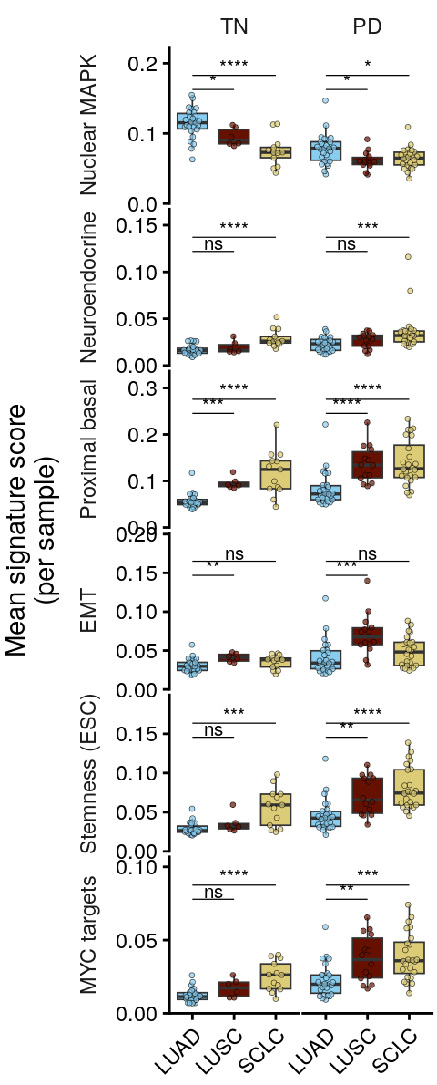
The heatmap pools cells. The two panels below work off sample-level means instead: for each
sample x lineage x timepoint with at least `MIN_CELLS_SIG` tumour cells, the mean of each
signature score.
```{r figs10efg-pseudobulk}
MIN_CELLS_SIG <- 5

# Signature -> group / display-name map, applying the same filters used in the heatmap.
sig_meta <- enframe(pth_list, name = "group", value = "signature") %>%
  unnest(signature) %>%
  distinct(signature, .keep_all = TRUE) %>%
  filter(!grepl("_epithelial$|TGFB", signature)) %>%
  mutate(
    source = case_when(
      grepl("^mp", signature)         ~ "Malignant Metaprograms",
      grepl("^TRAVAGLINI", signature) ~ "Travaglini",
      grepl("^HALLMARK_", signature)  ~ "Hallmark Pathways",
      .default = "Curated"),
    label = rename_pathway(signature)) %>%
  filter(!(grepl("MYC", signature, ignore.case = TRUE) & source == "Curated"))

sigs <- sig_meta$signature

df0 <- srt_ti@meta.data[, c("sample_id", "time_point", "lineage_class_coarse", sigs)]
df0[] <- lapply(df0, function(x) if (is.factor(x)) as.character(x) else x)

pb <- as_tibble(df0) %>%
  filter(time_point %in% c("TN", "PD"), !is.na(lineage_class_coarse)) %>%
  pivot_longer(all_of(sigs), names_to = "signature", values_to = "score") %>%
  group_by(sample_id, time_point, lineage = lineage_class_coarse, signature) %>%
  summarise(n_cells = n(), mean_score = mean(score), .groups = "drop") %>%
  filter(n_cells >= MIN_CELLS_SIG) %>%
  left_join(sig_meta, by = "signature") %>%
  mutate(time_point = factor(time_point, levels = c("TN", "PD")),
         lineage    = factor(lineage, levels = c("LUAD", "LUSC", "SCLC")))

# Samples contributing to each lineage x timepoint cell -- the n behind S10E and S10G.
pb %>% distinct(sample_id, time_point, lineage) %>% dplyr::count(time_point, lineage) %>%
  pivot_wider(names_from = lineage, values_from = n)
```
For every signature, the fraction of its genes (among those present in the data, since only
those can score) that fall inside the 179-gene panel. Signatures at or above
`PANEL_OVERLAP_MAX` are flagged panel-derived and excluded from the concordance test below.
```{r figs10efg-panel-overlap}
PANEL_OVERLAP_MAX <- 0.25   # >= this fraction of genes in the panel => "panel-derived"

panel_genes <- readxl::read_excel(here("paper_data", "supplemental_tables.xlsx"),
                                  sheet = "Table S7 - Histotime Features")$Gene %>%
  unique()
stopifnot(length(panel_genes) == 179)

# Geneset definitions: curated / Hallmark / Travaglini sets + malignant Tirosh metaprograms.
gs      <- read.table(here("paper_data", "egfr_pathways_v2.txt"), header = TRUE, sep = "\t")
mp_defs <- read.csv(here("paper_data", "tirosh_mps_67_natcan_2025.csv"), check.names = FALSE)
all_sets <- c(split(gs$Gene, gs$pathway), split(mp_defs$Gene, mp_defs$Geneset))

# Only the GIRARD/CCLE lineage sets have score-column names that differ from their geneset key.
sig_alias <- c(LUAD = "LUAD_GIRARD", LUSC = "LUSC_GIRARD", SCLC = "SCLC_CCLE")

# Only genes present in the data can contribute to a UCell score, so gate the denominator on
# the assay. The deposited object carries a single `RNA` assay.
universe <- rownames(srt_ti)
sig_key  <- function(s) if (s %in% names(all_sets)) s else unname(sig_alias[s])
sig_genes <- setNames(lapply(sigs, function(s) {
  k <- sig_key(s)
  if (is.na(k) || is.null(all_sets[[k]])) character(0)
  else intersect(unique(all_sets[[k]]), universe)
}), sigs)
stopifnot(all(lengths(sig_genes) > 0))   # every signature must resolve to a geneset

overlap_df <- tibble(signature = names(sig_genes)) %>%
  mutate(n_genes       = lengths(sig_genes[signature]),
         n_overlap     = map_int(sig_genes[signature], ~ length(intersect(.x, panel_genes))),
         frac_overlap  = n_overlap / n_genes,
         panel_derived = frac_overlap >= PANEL_OVERLAP_MAX) %>%
  left_join(sig_meta %>% dplyr::select(signature, label, group), by = "signature")

panel_indep_sigs <- overlap_df %>% filter(!panel_derived) %>% pull(signature)
```
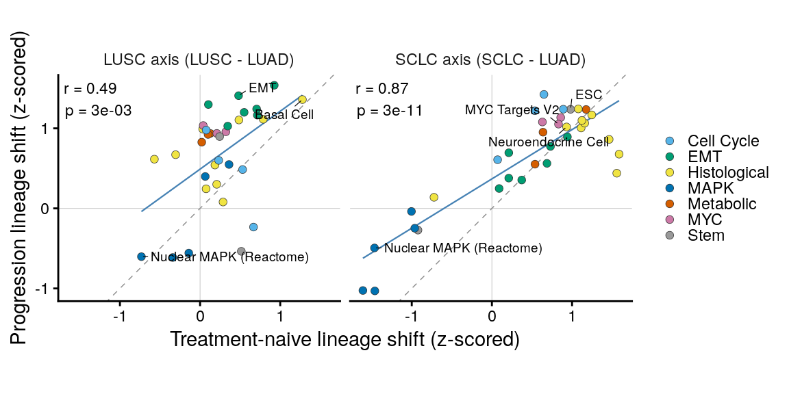
Each signature is z-scored across sample-level means, so signatures with different dynamic
ranges are comparable. Its lineage shift -- the mean z-score in LUSC-primed (or SCLC-primed)
samples minus that in LUAD samples -- is then computed separately at TN and at PD, and the two
are correlated. Only the panel-independent signatures enter the correlation.
```{r figs10e-lineage-leaning-tn-pd-concordance, fig.width = 6, fig.height = 3}
pb_z <- pb %>% group_by(signature) %>%
  mutate(mean_score = as.numeric(scale(mean_score))) %>% ungroup()

grp_means <- pb_z %>%
  group_by(signature, label, group, source, time_point, lineage) %>%
  summarise(m = mean(mean_score), .groups = "drop")

shifts <- grp_means %>%
  pivot_wider(names_from = lineage, values_from = m) %>%
  mutate(LUSC_shift = LUSC - LUAD, SCLC_shift = SCLC - LUAD) %>%
  dplyr::select(signature, label, group, source, time_point, LUSC_shift, SCLC_shift) %>%
  pivot_longer(c(LUSC_shift, SCLC_shift), names_to = "axis", values_to = "shift") %>%
  mutate(axis = sub("_shift", "", axis)) %>%
  pivot_wider(names_from = time_point, values_from = shift) %>%
  left_join(overlap_df %>% dplyr::select(signature, frac_overlap, panel_derived),
            by = "signature")

shifts_pi <- shifts %>% filter(!panel_derived)
stopifnot(dplyr::setequal(shifts_pi$signature, panel_indep_sigs))

# Per-signature correlation, reported on the panel.
cor_tab <- shifts_pi %>%
  group_by(axis) %>%
  summarise(r = cor(TN, PD), rho = cor(TN, PD, method = "spearman"),
            p = cor.test(TN, PD)$p.value, n = n(), .groups = "drop")
axis_labs <- c(LUSC = "LUSC axis (LUSC - LUAD)", SCLC = "SCLC axis (SCLC - LUAD)")
# Label only each axis's own fate-defining programmes -- the signatures called out in the text.
lab_map <- tibble::tribble(
  ~axis,  ~label,
  "SCLC", "Neuroendocrine Cell",
  "SCLC", "Nuclear MAPK (Reactome)",
  "SCLC", "ESC",
  "SCLC", "MYC Targets V2",
  "LUSC", "Basal Cell",
  "LUSC", "EMT",
  "LUSC", "Nuclear MAPK (Reactome)"
)

cor_ann <- cor_tab %>%
  mutate(lab = sprintf("r = %.2f\np = %s", r, format(p, digits = 1, scientific = TRUE)))

p_conc <- shifts_pi %>%
  ggplot(aes(TN, PD)) +
  geom_hline(yintercept = 0, linewidth = 0.2, colour = "grey80") +
  geom_vline(xintercept = 0, linewidth = 0.2, colour = "grey80") +
  geom_abline(slope = 1, intercept = 0, linetype = 2, linewidth = 0.25, colour = "grey55") +
  geom_smooth(method = "lm", se = FALSE, linewidth = 0.4, colour = "steelblue") +
  geom_point(aes(fill = group), shape = 21, size = 1.9, stroke = 0.2, colour = "grey20") +
  geom_text_repel(data = ~ dplyr::semi_join(.x, lab_map, by = c("axis", "label")),
                  aes(label = label), size = 2.5, min.segment.length = 0, segment.size = 0.2,
                  max.overlaps = Inf, box.padding = 0.3) +
  geom_text(data = cor_ann, aes(x = -Inf, y = Inf, label = lab), hjust = -0.1, vjust = 1.2,
            size = 3, inherit.aes = FALSE) +
  facet_wrap(~ axis, labeller = as_labeller(axis_labs)) +
  scale_fill_pander() +
  labs(x = "Treatment-naive lineage shift (z-scored)",
       y = "Progression lineage shift (z-scored)", fill = NULL) +
  coord_equal() +
  theme(legend.position = "right", legend.key.size = unit(3, "mm"),
        strip.background = element_blank(),
        panel.grid.minor = element_blank())

ggsave(p_conc, file = here("plots", "lineage_leaning_tn_pd_concordance.pdf"),
       width = 6, height = 3)
p_conc
```
## Figure S10F -- signature expression by lineage class and treatment state
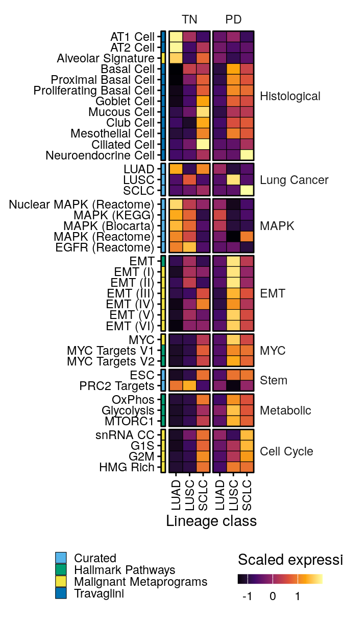
`DotPlotter()` wraps `Seurat::DotPlot()`; only the scaled-expression table it returns is kept.
MRD is dropped so the heatmap contrasts TN against PD directly.
```{r figs10efg-compute}
pth_df <- DotPlotter(
  srt_ti[, srt_ti$time_point != "MRD"],
  features       = pth_list,
  cluster_groups = FALSE,
  cluster_feats  = FALSE,
  group.by       = "lineage_class_coarse",
  split_by       = "time_point"
)$data
```
```{r figs10efg-wrangle}
# Tidy names, tag each signature by its source collection, and drop redundant MYC curated
# variants.
pth_df <- pth_df %>%
  filter(!grepl("_epithelial$", features.plot)) %>%
  filter(!grepl("TGFB", features.plot)) %>%
  mutate(pathway = rename_pathway(features.plot)) %>%
  mutate(
    pathway_source = case_when(
      grepl("^mp", features.plot)         ~ "Malignant Metaprograms",
      grepl("^TRAVAGLINI", features.plot) ~ "Travaglini",
      grepl("^HALLMARK_", features.plot)  ~ "Hallmark Pathways",
      features.plot %in% c("S.Score", "G2M.Score") ~ "Seurat",
      .default = "Curated"
    )
  ) %>%
  # The curated MYC sets duplicate the Hallmark MYC signal.
  filter(!(grepl("MYC", features.plot, ignore.case = TRUE) & pathway_source == "Curated")) %>%
  arrange(dplyr::desc(pathway_source), dplyr::desc(pathway))

pth_cat_order <- c("Histological", "Lung Cancer", "MAPK", "EMT", "MYC",
                   "Stem", "Metabolic", "Cell Cycle")

pth_order <- c(
  "G1S", "G2M", "G2M Score", "HMG Rich", "S Score",
  "EMT (I)", "EMT (II)", "EMT (III)", "EMT (IV)", "EMT (V)", "EMT (VI)",
  "LUAD", "LUSC", "SCLC",
  "AT1 Cell", "AT2 Cell", "Alveolar Signature", "Basal Cell", "Proximal Basal Cell",
  "Proliferating Basal Cell", "Goblet Cell", "Mucous Cell", "Club Cell", "Mesothelial Cell",
  "Ciliated Cell", "Neuroendocrine Cell", "MYC", "MYC Targets V1", "MYC Targets V2",
  "Glycolysis", "Oxidative Phosphorylation", "MTORC1", "ESC", "PRC2 Targets",
  "Nuclear MAPK (Reactome)", "MAPK (KEGG)", "MAPK (Biocarta)", "MAPK (Reactome)", "EGFR (Reactome)"
)

pth_df <- pth_df %>%
  mutate(
    pathway        = fct_relevel(pathway, rev(pth_order)),
    feature.groups = fct_relevel(feature.groups, pth_cat_order)
  )
```
```{r figs10f-lineage-leaning-signature-heatmap, fig.width = 3.5, fig.height = 6.3}
# Left strip: which collection each signature comes from.
p1 <- pth_df %>%
  ggplot(aes(x = "Pathway Source", y = pathway)) +
  geom_tile(aes(fill = pathway_source), color = "black") +
  scale_fill_pander() +
  scale_x_discrete(expand = c(0, 0)) +
  scale_y_discrete(expand = c(0, 0)) +
  theme(
    axis.line.x = element_blank(), axis.line.y = element_blank(),
    legend.position = "left", strip.background = element_blank(), strip.text = element_blank(),
    axis.text.x = element_blank(), axis.ticks.x = element_blank()
  ) +
  guides(x = guide_axis(angle = 90),
         fill = guide_legend(ncol = 1, keywidth = unit(3, "mm"), keyheight = unit(3, "mm"))) +
  facet_grid(feature.groups ~ ., scales = "free", space = "free") +
  labs(y = NULL, x = NULL, fill = NULL)

p2 <- pth_df %>%
  ggplot(aes(x = group.by, y = pathway)) +
  geom_tile(aes(fill = avg.exp.scaled), color = "black") +
  scale_fill_viridis_c(option = "inferno", breaks = c(-1, 0, 1)) +
  facet_grid(feature.groups ~ time_point, scales = "free", space = "free") +
  guides(x = guide_axis(angle = 90),
         fill = guide_colorbar(direction = "horizontal", title.position = "top",
                               label.position = "bottom", barwidth = unit(22, "mm"),
                               barheight = unit(2.5, "mm"))) +
  scale_x_discrete(expand = c(0, 0)) +
  scale_y_discrete(expand = c(0, 0)) +
  theme(
    axis.line = element_blank(), panel.border = element_blank(),
    strip.background.y = element_blank(),
    strip.text.y.right = element_text(angle = 0, hjust = 0),
    strip.background.x = element_blank(), strip.placement = "outside"
  ) +
  labs(y = NULL, x = "Lineage class", fill = "Scaled expression")

sig_heatplot <-
  (p1 + theme(plot.margin = margin(l = 0.25, r = 1, unit = "mm"))) +   # compact row labels
  (p2 + theme(plot.margin = margin(r = 0.25, unit = "mm"),
              axis.text.y = element_blank(), axis.ticks.y = element_blank())) +
  plot_layout(guides = "collect", ncol = 2, widths = c(0.05, 1)) +
  plot_annotation(theme = theme(legend.position = "bottom", legend.box = "horizontal",
                                legend.text = element_text(size = 6),
                                legend.title = element_text(size = 7))) &
  theme(panel.spacing = unit(0.8, "mm"),
        panel.border = element_rect(fill = NA, color = "black", linewidth = 0.5),
        legend.box.margin = margin()) &
  coord_cartesian(clip = "off")

ggsave(sig_heatplot, file = here("plots", "lineage_leaning_signature_heatmap.pdf"),
       width = 3.5, height = 6.3)
sig_heatplot
```
## Figure S10G -- sample-level scores for six fate programs
```{r figs10g-lineage-leaning-fate-signatures, fig.width = 2.5, fig.height = 6.2}
lin_cols <- colors$lineage_class_detailed[c("LUAD", "LUSC", "SCLC")]
lin_x    <- c(LUAD = 1, LUSC = 2, SCLC = 3)

sig_ord  <- c("Nuclear MAPK (Reactome)", "Neuroendocrine Cell", "Proximal Basal Cell",
              "EMT", "ESC", "MYC Targets V2")
# Concise strip labels (vertical, so they must stay short).
sig_labs <- c("Nuclear MAPK (Reactome)" = "Nuclear MAPK", "Neuroendocrine Cell" = "Neuroendocrine",
              "Proximal Basal Cell" = "Proximal basal", "EMT" = "EMT",
              "ESC" = "Stemness (ESC)", "MYC Targets V2" = "MYC targets")

box_df <- pb %>% filter(label %in% sig_ord) %>% mutate(label = factor(label, levels = sig_ord))
stopifnot(dplyr::setequal(levels(droplevels(box_df$label)), sig_ord))

stat_raw <- box_df %>%
  group_by(label, time_point) %>%
  rstatix::wilcox_test(mean_score ~ lineage,
                       comparisons = list(c("LUAD", "LUSC"), c("LUAD", "SCLC"))) %>%
  ungroup() %>%
  mutate(p.adj = p.adjust(p, method = "BH")) %>%
  rstatix::add_significance("p.adj")

row_max <- box_df %>% group_by(label) %>% summarise(ymax = max(mean_score), .groups = "drop")
brk_box <- stat_raw %>%
  left_join(row_max, by = "label") %>%
  mutate(x = lin_x[group1], xend = lin_x[group2],
         rung = if_else(group2 == "LUSC", 1, 2),
         y = ymax * (1.05 + 0.13 * (rung - 1)), lab = p.adj.signif)

p_box <- box_df %>%
  ggplot(aes(lineage, mean_score)) +
  geom_boxplot(aes(fill = lineage), outliers = FALSE, linewidth = 0.3, width = 0.72) +
  geom_quasirandom(aes(fill = lineage), size = 0.9, alpha = 0.7, colour = "black",
                   stroke = 0.2, pch = 21, width = 0.22) +
  geom_segment(data = brk_box, aes(x = x, xend = xend, y = y, yend = y),
               linewidth = 0.22, inherit.aes = FALSE) +
  geom_text(data = brk_box, aes(x = (x + xend) / 2, y = y, label = lab),
            vjust = -0.1, size = 2.7, inherit.aes = FALSE) +
  facet_grid(label ~ time_point, scales = "free_y", switch = "y",
             labeller = labeller(label = sig_labs)) +
  scale_fill_manual(values = lin_cols, guide = "none") +
  scale_x_discrete(expand = expansion(add = 0.55)) +
  scale_y_continuous(expand = expansion(mult = c(0, 0.22)), n.breaks = 4) +
  expand_limits(y = 0) +
  labs(x = NULL, y = "Mean signature score\n(per sample)") +
  guides(x = guide_axis(angle = 45)) +
  coord_cartesian(clip = "off") +
  theme(strip.background = element_blank(), strip.placement = "outside",
        panel.spacing.x = unit(0.6, "mm"), panel.spacing.y = unit(0.8, "mm"),
        panel.grid.minor = element_blank(),
        strip.clip = "off",
        plot.margin = margin(2, 2, 2, 2))

ggsave(p_box, file = here("plots", "lineage_leaning_fate_signatures.pdf"),
       width = 2.5, height = 6.2)
p_box
```
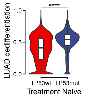
## Figure S10H -- LUAD deprogramming in TP53-mutant vs wildtype TN
```{r figs10h-tp53mut-tn-luad-dediff, fig.width = 1.75, fig.height = 2}
p <- srt_ti@meta.data %>%
  mutate(TP53mut = case_when(
    has_impact == F ~ "NA",
    tp53mut ~ "TP53mut",
    !tp53mut ~ "TP53wt",
    .default = "Other"
  )) %>%
  filter(time_point == "TN" & TP53mut != "NA") %>%
  ggplot(aes(x = fct_rev(TP53mut), y = luad_dediff)) +
  geom_violin(scale = "width", aes(fill = TP53mut), show.legend = F) +
  scale_fill_aaas() +
  geom_boxplot(width = 0.2, outliers = F) +
  scale_y_continuous(breaks = c(0, 0.5, 1)) +
  guides(y = guide_axis(cap = "both"),
         x = guide_axis(cap = "both")) +
  ggpubr::geom_pwc(label = "p.signif", tip.length = 0, vjust = 0.5) +
  coord_cartesian(clip = "off") +
  labs(x = "Treatment Naive", y = "LUAD dedifferentiation")
p
ggsave(p, file = here("plots", "TP53mut_TN_luad_dediff.pdf"), width = 1.75, height = 2)
```
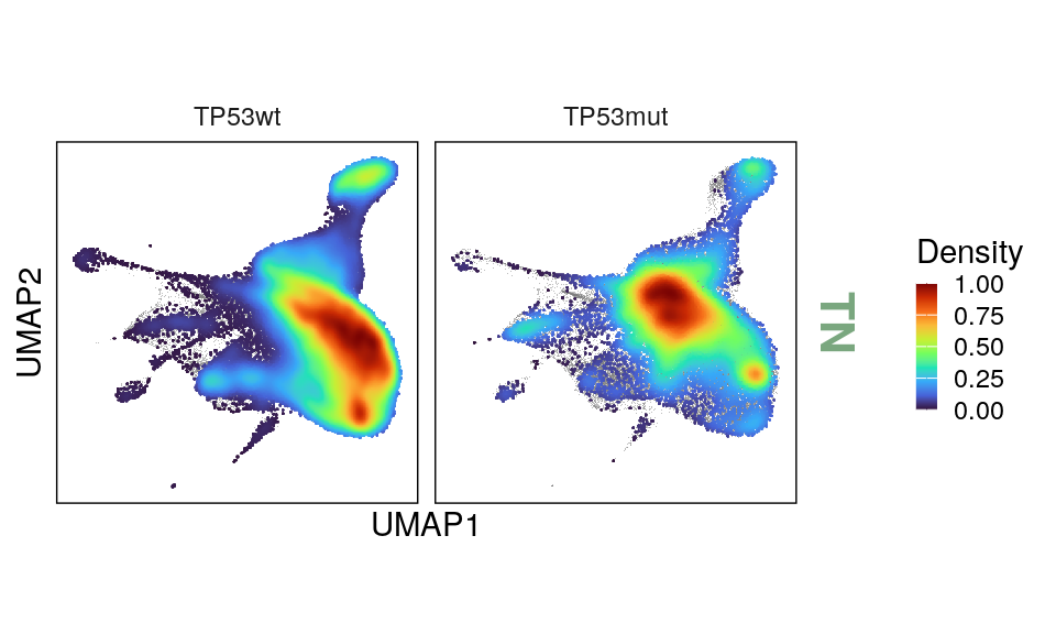
## Figure S10I -- TP53-mutant vs wildtype tumor cell density
```{r}
library(ggtext)
df <- FetchData(srt_epi, vars = c("time_point", "is_tumor_cell", "cell_type", "umap_1", "umap_2", "tp53mut", "rb1mut", "has_impact")) %>%
  dplyr::rename("UMAP1" = "umap_1", "UMAP2" = "umap_2") %>%
  filter(is_tumor_cell) %>%
  mutate(tp53mut = case_when(
    has_impact == F ~ "NA",
    tp53mut ~ "TP53mut",
    !tp53mut ~ "TP53wt",
    .default = "Other"
  ))
# Group by timepoint and calculate scaled density per group
df <- df %>%
  group_by(time_point, cell_type, tp53mut) %>%
  mutate(density = get_density(UMAP1, UMAP2, n = 500)) %>%
  mutate(density_scaled = standardize(density))

df$time_point_col <- factor(df$time_point,
  levels = levels(df$time_point),
  labels = glue("<b style='color:{colors$time_point[levels(df$time_point)]}'>{levels(df$time_point)}</b>")
)
```
```{r figs10i-tp53mut-tumor-cell-density-tnonly, fig.width = 5, fig.height = 3}
# TN only
p <- df %>%
  filter(tp53mut != "NA", time_point == "TN") %>%
  ungroup() %>%
  arrange((density_scaled)) %>%
  ggplot(aes(x = UMAP1, y = UMAP2)) +
  scattermore::geom_scattermore(data = dplyr::select(df_raw_background, -time_point), color = "grey50", alpha = 0.5) +
    scattermore::geom_scattermore(aes(color = density_scaled), pointsize = 3, pixels = c(512, 512)) +
  facet_grid(time_point_col ~ fct_rev(tp53mut)) +
  scale_color_gradientn(colours = viridis::turbo(10), name = "Density") +
  guides(color = guide_colorbar(keywidth = 0.5, keyheight = 3)) +
  theme(
    strip.background = element_blank(),
    strip.text.y = element_markdown(size = 16),
    aspect.ratio = 1, panel.background = element_rect(fill = NA, color = "black"),
    plot.title = element_text(hjust = 0.5, size = 18),
    axis.line = element_blank(),
    axis.ticks = element_blank(),
    axis.text = element_blank()
  ) +
  labs(x = "UMAP1", y = "UMAP2")
ggsave(p, file = here("plots", "TP53mut_tumor_cell_density_TNonly.pdf"), width = 5, height = 3)
p
```
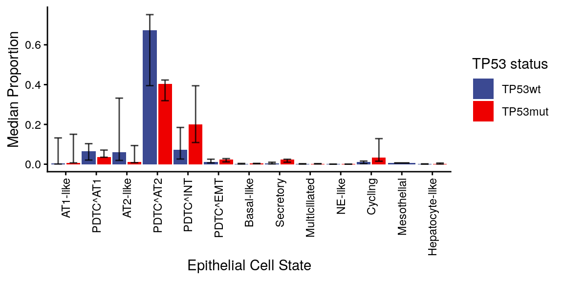
## Figure S10J -- epithelial state proportions by TP53 status
```{r figs10j-tp53mut-tn-epi-type-proportions, fig.width = 6, fig.height = 3}
prop_df <- srt_ti@meta.data %>%
  mutate(TP53mut = case_when(
    has_impact == F ~ "NA",
    tp53mut ~ "TP53mut",
    !tp53mut ~ "TP53wt",
    .default = "Other"
  )) %>%
  filter(time_point == "TN" & TP53mut != "NA", is_tumor_cell) %>%
  add_count(sample_id, name = "n_samp") %>%
  add_count(sample_id, cell_type_epi, name = "n_ct") %>%
  mutate(prop = n_ct / n_samp) %>%
  distinct(sample_id, TP53mut, cell_type_epi, prop)

p <- prop_df %>%
  ggplot(aes(x = cell_type_epi, y = prop)) +
  stat_summary(geom = "bar", fun = "median", aes(fill = fct_rev(TP53mut)), position = position_dodge(width = 1)) +
  geom_errorbar(aes(group = fct_rev(TP53mut)),
      stat = "summary", color = "black", alpha = 0.75, width = 0.5,
    fun.min = function(z) {
      quantile(z, 0.25)
    },
    fun.max = function(z) {
      quantile(z, 0.75)
    },
    fun = median, position = position_dodge(width = 1)) +
  guides(x = guide_axis(angle = 90)) +
  labs(y = "Median Proportion", x = "Epithelial Cell State", fill = "TP53 status") +
  scale_fill_aaas()
ggsave(p, file = here("plots", "TP53mut_TN_epi_type_proportions.pdf"), width = 6, height = 3)
p
```