---
title: "Figure reproduction -- Xenium spatial cohort"
author: "Matthew Zatzman"
execute:
warning: false
error: false
format:
html:
code-fold: true
code-tools: true
toc: true
---
```{r setup}
#| output: false
library(tidyverse)
library(glue)
library(Seurat)
library(ggsci)
library(ggthemes)
library(patchwork)
library(ggh4x)
library(legendry)
library(here)
devtools::load_all(here())

options(future.globals.maxSize = Inf)
set.seed(42)
options(scipen = 0)

colors <- load_colors()
colors$site_of_tissue_simple <- xenium_site_palette()
markers <- load_markers()
patients <- paste0("XE", 1:5)

# Swimmer rows read top-to-bottom XE1..XE5, so the y-axis factor runs the other way.
pt_order <- paste0("XE", 5:1)

# Every panel here is written to plots/xenium/, which is not in the repo.
dir.create(here("plots", "xenium"), recursive = TRUE, showWarnings = FALSE)
stopifnot(dir.exists(here("plots", "xenium")))
```
## Ingest
```{r ingest-tables}
supp <- here("paper_data", "supplemental_tables.xlsx")

blank_na <- function(x) ifelse(as.character(x) == "NA", NA_character_, as.character(x))
as_num <- function(x) suppressWarnings(as.numeric(blank_na(x)))

# --- Table S9: per-sample Xenium metadata (10 rows, one per Xenium section) ------------
xe_meta <- suppressMessages(readxl::read_excel(supp, sheet = "Table S9 - Xenium Metadata")) %>%
  mutate(
    across(c(egfr_mutation, site_of_tissue_simple, procedure_type), blank_na),
    # Named one by one, not by starts_with(): facets_wgd is also a facets_ column but holds
    # "TRUE"/"FALSE"/"NA", and as_num() would blank all three -- painting the whole S11A WGD
    # strip na.value grey.
    across(c(facets_purity, facets_ploidy, facets_fga, facets_tmb), as_num),
    facets_wgd = as.logical(blank_na(facets_wgd)),
    patient_id = factor(patient_id, levels = patients),
    timepoint = factor(timepoint, levels = c("TN", "PD"))
  )
stopifnot(is.numeric(xe_meta$facets_purity), is.logical(xe_meta$facets_wgd),
          sum(!is.na(xe_meta$facets_wgd)) == 9L)
stopifnot(nrow(xe_meta) == 10L, sum(xe_meta$has_impact) == 9L)

# --- Table S10: IMPACT alterations, Xenium-matched samples only (70 rows) --------------
xe_muts <- suppressMessages(readxl::read_excel(supp, sheet = "Table S10 - Xenium IMPACT Muts")) %>%
  mutate(
    across(c(gene, mut_class, mutation_type_simple, HGVSp_Short, source), blank_na),
    across(starts_with("ccf_"), as_num),
    sample_id = paste0(patient_id, "_", timepoint)
  )
stopifnot(nrow(xe_muts) == 70L, sum(!is.na(xe_muts$ccf_expected_copies)) == 40L)

# --- FACETS bundle: per-sample type + per-segment copy number -------------------------
facets <- readRDS(here("paper_data", "xenium_impact_facets.rds"))
stopifnot(nrow(facets$samples) == 9L, all(facets$segments$chrom %in% 1:23))

# --- De-identified clinical timeline (years from diagnosis) ---------------------------
tl <- readRDS(here("paper_data", "xenium_clinical_timeline.rds"))
stopifnot(setequal(names(tl), c("tx_lines", "patient_summary", "radiation")))
```
```{r ingest-check}
xe_meta %>%
  dplyr::select(sample_id, has_impact, site_of_tissue_simple, procedure_type, egfr_mutation)
```
```{r ingest}
obj <- readRDS(here("paper_data", "xenium_seurat.rds"))
DefaultAssay(obj) <- "Xenium"
srt <- obj

# The ten Fig 6E crops, stored on the object under these names. `x`/`y` are the axis
# limits each panel is drawn to, in microns.
crops_spec <- list(
  XE1_TN_crop = list(x = c(7000, 7200), y = c(8400, 8600)),
  XE1_PD_crop = list(x = c(6700, 6900), y = c(2400, 2600)),
  XE2_TN_crop = list(x = c(6300, 6500), y = c(7900, 8100)),
  XE2_PD_crop = list(x = c(3050, 3250), y = c(1600, 1800)),
  XE3_TN_crop = list(x = c(4700, 4900), y = c(3700, 3900)),
  XE3_PD_crop = list(x = c(2800, 3000), y = c(1050, 1250)),
  XE4_TN_crop = list(x = c(3158, 3358), y = c(3012, 3212)),
  XE4_PD_crop = list(x = c(1800, 2000), y = c(1930, 2130)),
  XE5_TN_crop = list(x = c(2700, 2900), y = c(1600, 1800)),
  XE5_PD_crop = list(x = c(6800, 7000), y = c(1600, 1800))
)

egfr_probes <- c("EGFR-ALT-2496:", "EGFR-ALT-2650:A", "EGFR-ALT-2651:C", "EGFR-ALT-2834:G",
                 "EGFR-WT-2496", "EGFR-WT-2650-2651", "EGFR-WT-2834")
srt_epi <- obj[setdiff(rownames(obj), egfr_probes), obj$is_epithelial]
srt_epi@images <- list()
srt_epi <- NormalizeData(srt_epi, verbose = FALSE)
stopifnot(nrow(srt_epi) == 382L)

# `umap_tumor` is populated on the is_tumor_cell population only, so each per-patient
# object carries its own slice of it.
srt_pts <- setNames(lapply(patients, function(pat) {
  o <- obj[, obj$is_tumor_cell & obj$patient_id == pat]
  o@images <- list()                  # nothing downstream of srt_pts uses FOVs
  o[["umap"]] <- o[["umap_tumor"]]
  o$timepoint <- as.character(o$timepoint)
  o
}), patients)

knn_results <- obj@meta.data %>% filter(is_tumor_cell) %>%
  transmute(cell_id, patient_id = as.character(patient_id),
            timepoint = as.character(timepoint),
            pd_neighbor_frac, pd_proximity, pd_like_tn)

percell_sims <- obj@meta.data %>% filter(is_tumor_cell) %>%
  transmute(cell_id, patient_id = as.character(patient_id),
            category = pd_category, pd_axis)

# Two side files ship with the object because neither is regenerable from it:
#   pt_sp.txt.gz             the Fig S12C specificity values. calc_snn_specificity()
#                            subsamples at 10% with no seed, so a recompute differs.
#   XE1_TN_select_region.csv the hand-drawn Xenium Explorer region restricting the XE1_TN
#                            panel of Fig S13D.
pt_sp_file      <- here("paper_data", "pt_sp.txt.gz")
xe1_region_file <- here("paper_data", "XE1_TN_select_region.csv")
stopifnot(file.exists(pt_sp_file), file.exists(xe1_region_file))

# The three lineage signatures behind the deposited *_score columns. Fig 6F reads the
# names, Fig S13C the members.
lung_lineage_genes <- list(
  alveolar = c("SFTPC","SFTPB","SFTPD","SFTA2","NAPSA","NKX2-1","ETV5","PLA2G4F","AGER","HOPX","PDPN","CLIC5"),
  basal_squamous = c("TP63","SOX2","KRT5","KRT14","KRT6A","KRT13","KRT15","KRT16","KRT17","DSG3","ITGB4","SLC2A1","TP73","S100A7","PI3"),
  neuroendocrine = c("ASCL1","NEUROD1","SYP","CHGA","NCAM1")
)
```
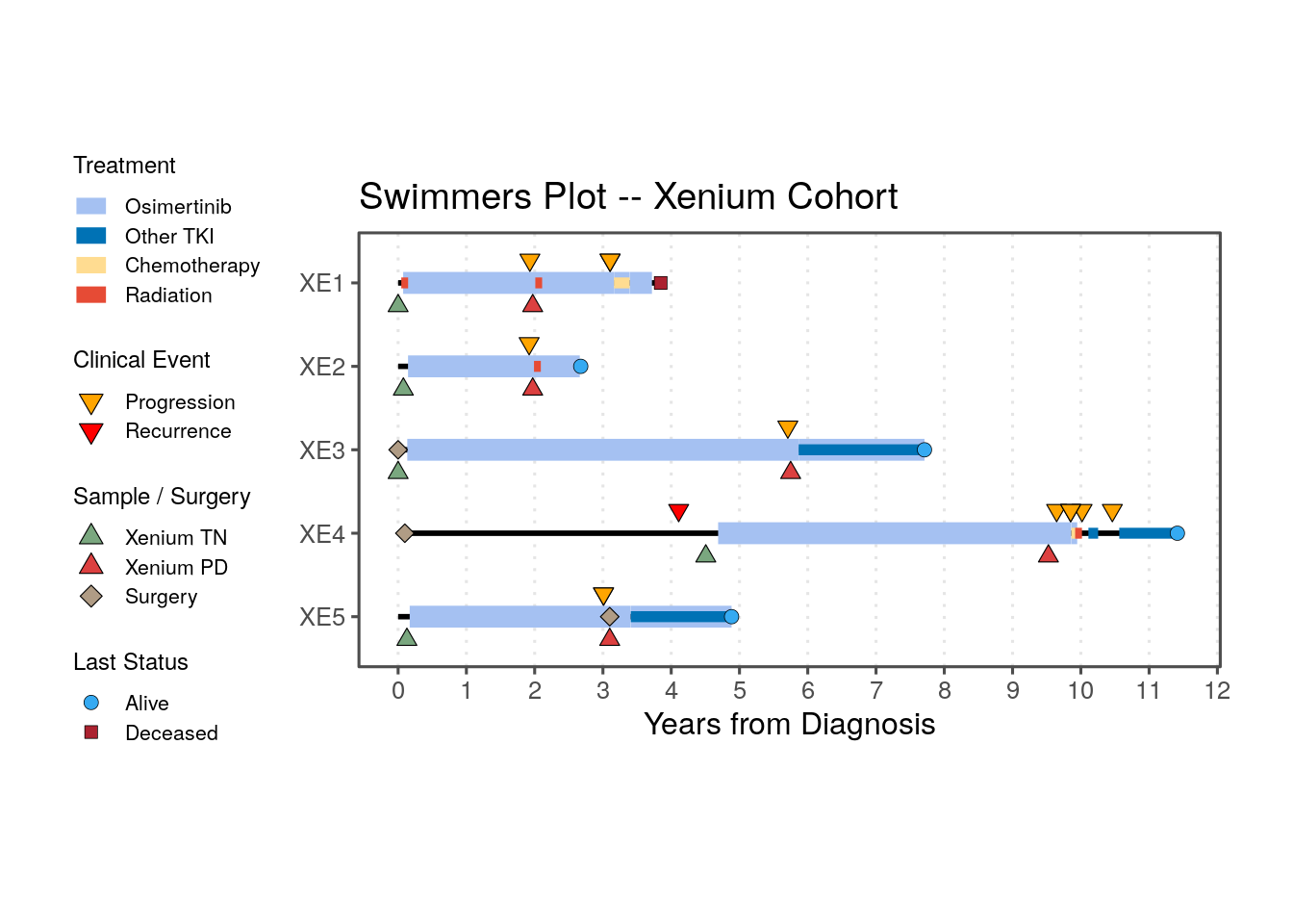
## Fig 6A — swimmer plot
```{r swimmer-data}
tx_lines <- tl$tx_lines %>% mutate(patient_id = factor(patient_id, levels = pt_order))
patient_summary <- tl$patient_summary %>%
  mutate(patient_id = factor(patient_id, levels = pt_order))
radiation_events <- tl$radiation %>%
  mutate(patient_id = factor(patient_id, levels = pt_order))

# Osimertinib carries the thick backbone, everything else is drawn thinner over it.
# Combination regimens were split upstream into an osimertinib row plus a partner row, so
# `regimen_class` is always a single modality here.
tx_valid <- filter(tx_lines, !is.na(tx_start_yr), !is.na(tx_end_yr))
tx_osi <- filter(tx_valid, regimen_class == "Osimertinib")
tx_other <- filter(tx_valid, regimen_class != "Osimertinib")

tx_colors <- c(
  "Osimertinib" = "#a5c1f2",
  "Other TKI" = "#0072B5",
  "Chemotherapy" = "#FFDC91",
  "Radiation" = "#E64B35"
)
# Every regimen class in the data must have a colour, or the bar silently disappears.
stopifnot(all(c(tx_valid$regimen_class, radiation_events$regimen_class) %in% names(tx_colors)))
```
```{r swimmer, fig.width = 7, fig.height = 5}
tri_size <- 2.5
tri_stroke <- 0.3
tri_nudge <- 0.275
kwd <- 1
kht <- 0.8

swimmers_plot <- ggplot() +
  # FOLLOW-UP BAR
  geom_segment(
    data = patient_summary,
    aes(x = 0, xend = fu_yr, y = patient_id, yend = patient_id),
    linewidth = 1, color = "black"
  ) +
  # OSIMERTINIB (thick backbone)
  geom_segment(
    data = tx_osi,
    aes(x = tx_start_yr, xend = tx_end_yr, y = patient_id, yend = patient_id, color = regimen_class),
    linewidth = 4
  ) +
  # OTHER SYSTEMIC TREATMENTS (thinner)
  geom_segment(
    data = tx_other,
    aes(x = tx_start_yr, xend = tx_end_yr, y = patient_id, yend = patient_id, color = regimen_class),
    linewidth = 2
  ) +
  # RADIATION (single-day courses get a 0.1 yr minimum so they remain visible)
  geom_segment(
    data = radiation_events,
    aes(
      x = rt_start_yr, xend = pmax(rt_end_yr, rt_start_yr + 0.1),
      y = patient_id, yend = patient_id, color = regimen_class
    ),
    linewidth = 2
  ) +
  scale_color_manual(
    name = "Treatment", values = tx_colors,
    breaks = c("Osimertinib", "Other TKI", "Chemotherapy", "Radiation"),
    guide = guide_legend(override.aes = list(linewidth = 3), order = 1, keywidth = kwd, keyheight = kht)
  ) +
  # CLINICAL EVENTS (downward triangles, nudged up)
  geom_point(
    data = filter(tx_lines, !is.na(prog_yr)),
    aes(x = prog_yr, y = patient_id, fill = "Progression"),
    size = tri_size, stroke = tri_stroke, pch = 25,
    position = position_nudge(y = tri_nudge)
  ) +
  geom_point(
    data = filter(patient_summary, !is.na(recurrence_yr)),
    aes(x = recurrence_yr, y = patient_id, fill = "Recurrence"),
    size = tri_size, stroke = tri_stroke, pch = 25,
    position = position_nudge(y = tri_nudge)
  ) +
  scale_fill_manual(
    name = "Clinical Event",
    values = c("Progression" = "orange", "Recurrence" = "red"),
    limits = c("Progression", "Recurrence"),
    guide = guide_legend(override.aes = list(size = 3), order = 2, keywidth = kwd, keyheight = kht)
  ) +
  ggnewscale::new_scale_fill() +
  # SPECIMEN COLLECTION (upward triangles, nudged down) + SURGERY (diamond)
  geom_point(
    data = filter(patient_summary, !is.na(tn_sample_yr)),
    aes(x = tn_sample_yr, y = patient_id, fill = "Xenium TN"),
    size = tri_size, stroke = tri_stroke, pch = 24,
    position = position_nudge(y = -tri_nudge)
  ) +
  geom_point(
    data = filter(patient_summary, !is.na(pd_sample_yr)),
    aes(x = pd_sample_yr, y = patient_id, fill = "Xenium PD"),
    size = tri_size, stroke = tri_stroke, pch = 24,
    position = position_nudge(y = -tri_nudge)
  ) +
  geom_point(
    data = filter(patient_summary, !is.na(resection_yr)),
    aes(x = resection_yr, y = patient_id, fill = "Surgery"),
    size = tri_size, stroke = tri_stroke, pch = 23
  ) +
  scale_fill_manual(
    name = "Sample / Surgery",
    values = c("Xenium TN" = "#7aa77f", "Xenium PD" = "#dc4040", "Surgery" = "#B09C85"),
    limits = c("Xenium TN", "Xenium PD", "Surgery"),
    guide = guide_legend(override.aes = list(size = 3), order = 3, keywidth = kwd, keyheight = kht)
  ) +
  ggnewscale::new_scale_fill() +
  # LAST STATUS
  geom_point(
    data = patient_summary,
    aes(
      x = fu_yr, y = patient_id,
      fill = ifelse(alive, "Alive", "Deceased"),
      shape = ifelse(alive, "Alive", "Deceased")
    ),
    size = 2.5, stroke = 0.2
  ) +
  scale_shape_manual(
    name = "Last Status",
    values = c("Alive" = 21, "Deceased" = 22),
    guide = guide_legend(order = 4, keywidth = kwd, keyheight = kht)
  ) +
  scale_fill_manual(
    name = "Last Status",
    values = c("Alive" = "#35aaf2", "Deceased" = "#ab2230"),
    guide = guide_legend(order = 4, keywidth = kwd, keyheight = kht)
  ) +
  scale_x_continuous(breaks = seq(0, 20, by = 1), expand = expansion(mult = c(0.05, 0.05))) +
  guides(x = guide_axis(cap = "both"), y = guide_axis(cap = "both")) +
  labs(x = "Years from Diagnosis", y = NULL, title = "Swimmers Plot -- Xenium Cohort") +
  theme_few() +
  theme(
    legend.position = "left",
    legend.spacing.y = unit(15, "pt"),
    legend.margin = margin(0, 0, 0, 0),
    legend.box.spacing = unit(15, "pt"),
    legend.title = element_text(size = 9),
    legend.text = element_text(size = 8),
    panel.grid.major.x = element_line(color = "grey90", linetype = "dotted"),
    plot.margin = margin(25, 10, 25, 10, unit = "mm")
  ) +
  coord_cartesian(clip = "off")

ggsave(swimmers_plot,
  filename = here("plots", "xenium", "swimmers_plot.pdf"),
  width = 6, height = 5
)
swimmers_plot
```
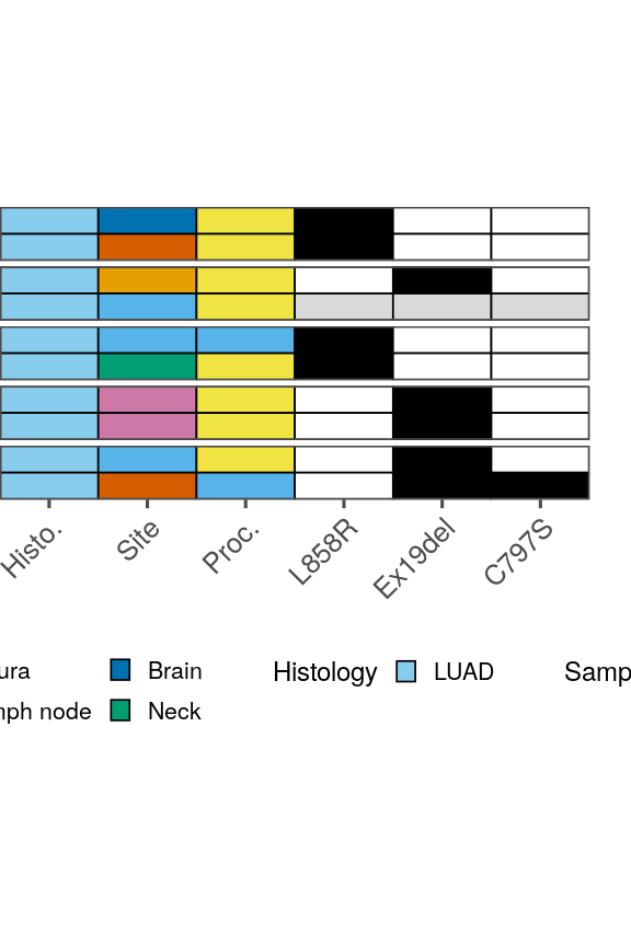
## Fig 6B — sample annotation tiles
```{r annot-tiles, fig.width = 3, fig.height = 4.5}
meta_xe_annot <- xe_meta %>%
  mutate(patient_id = factor(as.character(patient_id), levels = rev(pt_order)))

x_cats <- c("Histo.", "Site", "Proc.", "L858R", "Ex19del", "C797S")

# XE2_PD has no matched IMPACT sample, so Table S9 reports its EGFR allele as NA
has_allele <- function(pattern, x) ifelse(is.na(x), NA, grepl(pattern, x))
allele_pal <- c("TRUE" = "black", "FALSE" = "white")
stopifnot(
  all(na.omit(meta_xe_annot$site_of_tissue_simple) %in% names(colors$site_of_tissue_simple)),
  all(na.omit(meta_xe_annot$procedure_type) %in% c("Resection", "Biopsy"))
)

meta_annot_pl <- ggplot(meta_xe_annot, aes(y = fct_rev(timepoint))) +
  # Histology -- the Xenium cohort is LUAD throughout (Table S9, tumor_stage IV LUAD)
  geom_tile(aes(x = "Histo.", fill = "LUAD"), color = "black", linewidth = 0.3) +
  scale_fill_manual(
    name = "Histology", values = colors$histology_predominant_short,
    guide = guide_legend(keywidth = 0.5, keyheight = 0.5, order = 0)
  ) +
  ggnewscale::new_scale_fill() +
  geom_tile(aes(x = "Site", fill = site_of_tissue_simple), color = "black", linewidth = 0.3) +
  scale_fill_manual(
    name = "Tissue Site", values = colors$site_of_tissue_simple,
    breaks = unique(names(colors$site_of_tissue_simple)),
    guide = guide_legend(keywidth = 0.5, keyheight = 0.5, order = 1)
  ) +
  ggnewscale::new_scale_fill() +
  geom_tile(aes(x = "Proc.", fill = procedure_type), color = "black", linewidth = 0.3) +
  scale_fill_manual(
    name = "Sample Type",
    values = c("Resection" = "#56B4E9", "Biopsy" = "#F0E442"),
    guide = guide_legend(keywidth = 0.5, keyheight = 0.5)
  ) +
  ggnewscale::new_scale_fill() +
  # EGFR alleles. The exon-19 deletions (E746_A750del, E746_S752delinsV,
  # E746_T751delinsVP) are collapsed into one Ex19del column.
  geom_tile(aes(x = "L858R", fill = has_allele("L858R", egfr_mutation)),
    color = "black", linewidth = 0.3, show.legend = FALSE
  ) +
  geom_tile(aes(x = "Ex19del", fill = has_allele("^E746_", egfr_mutation)),
    color = "black", linewidth = 0.3, show.legend = FALSE
  ) +
  geom_tile(aes(x = "C797S", fill = has_allele("C797S", egfr_mutation)),
    color = "black", linewidth = 0.3, show.legend = FALSE
  ) +
  scale_fill_manual(values = allele_pal, na.value = "grey85") +
  scale_x_discrete(limits = x_cats, expand = c(0, 0), position = "bottom") +
  scale_y_discrete(expand = c(0, 0), position = "right") +
  facet_grid(patient_id ~ .) +
  theme_few() +
  labs(y = NULL, x = NULL) +
  guides(x = guide_axis(angle = 45)) +
  theme(
    axis.text.y = element_blank(),
    axis.ticks.y = element_blank(),
    strip.text.y = element_blank(),
    strip.background = element_blank(),
    legend.position = "bottom",
    legend.title = element_text(size = 9),
    legend.text = element_text(size = 8),
    panel.spacing.y = unit(2, "pt"),
    plot.margin = margin(25, 5, 25, 0, unit = "mm")
  )

ggsave(meta_annot_pl,
  filename = here("plots", "xenium", "sample_annotation_tiles.pdf"),
  width = 3, height = 4.5
)
meta_annot_pl
```
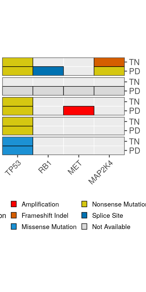
## Fig 6B — resistance mini-oncoprint
```{r mini-oncoprint, fig.width = 2.5, fig.height = 5}
mini_onco_genes <- c("MAP2K4", "MET", "RB1", "TP53")

# Table S10 is the alteration-to-section join already made, keyed on patient_id /
# timepoint.
mini_onco_df <- xe_muts %>%
  filter(gene %in% mini_onco_genes) %>%
  distinct(patient_id, timepoint, gene, mut_class) %>%
  # One class per gene x section: Amp > Del > truncating > missense.
  mutate(mut_priority = case_when(
    mut_class == "Amplification" ~ 1,
    mut_class == "Deep Deletion" ~ 2,
    mut_class %in% c("Nonsense Mutation", "Frameshift Indel") ~ 3,
    mut_class == "Missense Mutation" ~ 4,
    .default = 5
  )) %>%
  group_by(patient_id, timepoint, gene) %>%
  dplyr::slice_min(mut_priority, n = 1) %>%
  ungroup() %>%
  dplyr::select(patient_id, timepoint, gene, mut_class) %>%
  mutate(across(c(patient_id, timepoint), as.character))

# As with the allele tiles above: XE2_PD is "not assessed", not "no alteration", and gets a
# separate "Not Available" key in the same na.value grey.
mini_na_df <- xe_meta %>%
  filter(!has_impact) %>%
  dplyr::transmute(patient_id = as.character(patient_id),
                   timepoint = as.character(timepoint)) %>%
  tidyr::expand_grid(gene = mini_onco_genes) %>%
  mutate(mut_class = "Not Available")

mini_tiles <- bind_rows(mini_onco_df, mini_na_df)
mini_mut_pal <- c(colors$mutations, "Not Available" = "grey85")
# "Not Available" last so it closes the two-column legend, as placed.
mut_levels <- c(sort(setdiff(mini_tiles$mut_class, "Not Available")), "Not Available")
stopifnot(all(mut_levels %in% names(mini_mut_pal)))

# Background grid: one tile per section x gene, painted "assessed, no alteration".
mini_grid <- expand.grid(
  patient_id = patients,
  timepoint = c("TN", "PD"),
  gene = mini_onco_genes,
  stringsAsFactors = FALSE
)

# Facets read XE1..XE5 downwards, TN over PD within each, matching the swimmer's rows.
mini_grid$patient_id <- factor(mini_grid$patient_id, levels = patients)
mini_tiles$patient_id <- factor(mini_tiles$patient_id, levels = patients)
mini_grid$timepoint <- factor(mini_grid$timepoint, levels = c("TN", "PD"))
mini_tiles$timepoint <- factor(mini_tiles$timepoint, levels = c("TN", "PD"))
mini_tiles$mut_class <- factor(mini_tiles$mut_class, levels = mut_levels)

p_mini_onco <- ggplot() +
  geom_tile(
    data = mini_grid, aes(x = gene, y = fct_rev(timepoint)),
    fill = "#ECECEC", color = "white", linewidth = 0.3
  ) +
  geom_tile(
    data = mini_tiles, aes(x = gene, y = fct_rev(timepoint), fill = mut_class),
    color = "black", linewidth = 0.3, height = 1, width = 1
  ) +
  scale_fill_manual(
    name = "Mutation", values = mini_mut_pal, drop = TRUE,
    guide = guide_legend(keywidth = 0.5, keyheight = 0.5)
  ) +
  scale_x_discrete(limits = rev(mini_onco_genes), expand = c(0, 0), position = "bottom") +
  scale_y_discrete(expand = c(0, 0), position = "right") +
  facet_grid(patient_id ~ ., switch = "y") +
  theme_few() +
  labs(x = NULL, y = NULL) +
  guides(
    x = guide_axis(angle = 45),
    fill = guide_legend(ncol = 2, keywidth = 0.5, keyheight = 0.5)
  ) +
  theme(
    axis.text.y = element_text(size = 10),
    strip.text.y = element_blank(),
    strip.background = element_blank(),
    legend.position = "bottom",
    legend.title = element_text(size = 9),
    legend.text = element_text(size = 8),
    panel.spacing.y = unit(2, "pt"),
    plot.margin = margin(25, 2.5, 25, 1, unit = "mm")
  )

ggsave(p_mini_onco,
  filename = here("plots", "xenium", "resistance_mini_oncoprint.pdf"),
  width = 2.5, height = 5
)
p_mini_onco
```
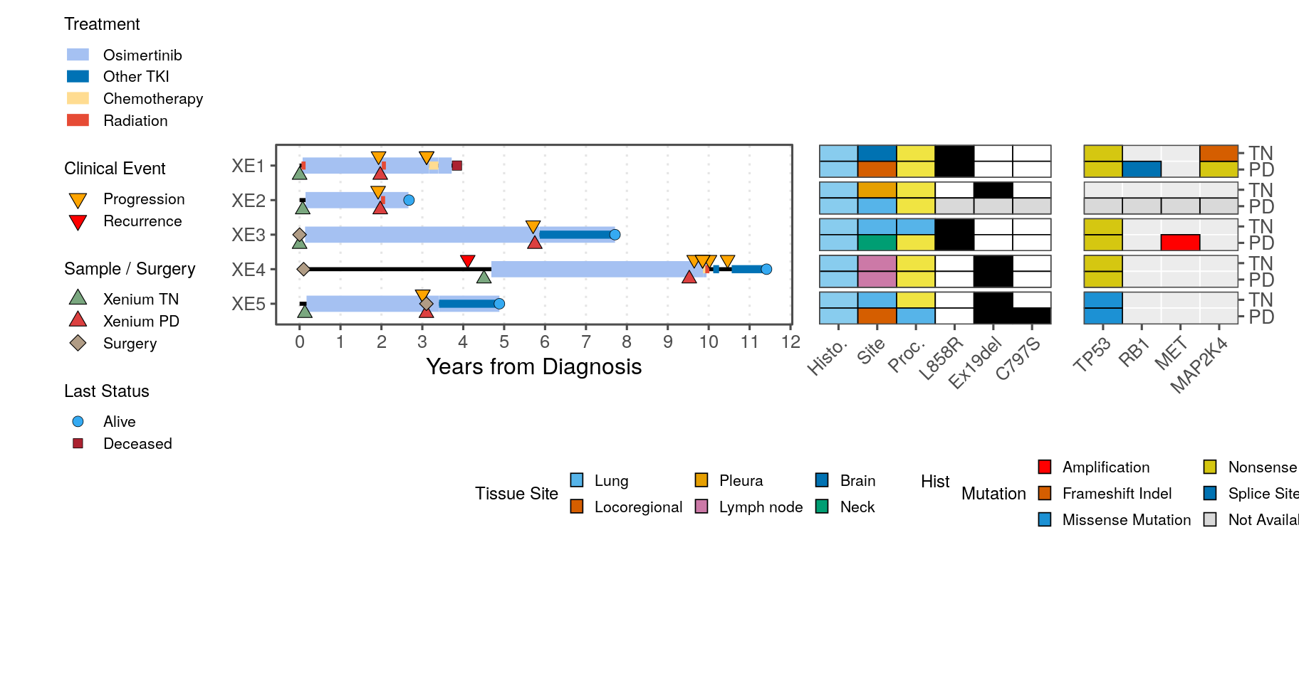
## Fig 6A + 6B assembled
```{r swimmer-combined, fig.width = 9.5, fig.height = 5}
swm_pl_cmb <- swimmers_plot +
  theme(
    plot.title = element_blank(),
    plot.margin = margin(25, 5, 25, 10, unit = "mm")
  )

swimmers_combined <- free(swm_pl_cmb, type = "label", side = "b") +
  meta_annot_pl +
  p_mini_onco +
  plot_layout(widths = c(2, 0.9, 0.6))

ggsave(swimmers_combined,
  filename = here("plots", "xenium", "swimmers_annotated.pdf"),
  width = 9.5, height = 5
)
swimmers_combined
```
## Backbone — fast_wilcox TN-vs-PD DE engine (Fig 6C, 6D, 6F)
```{r}
fts <- rownames(srt_epi)
df_all_fts <- FetchData(srt_epi[, srt_epi$cell_type_coarse == "Tumor"], vars = c("cell_id", "patient_id", "nCount_RNA", "mut_pos_cell", "timepoint", "cell_type_coarse", fts))
df_all_fts$timepoint <- fct_relevel(df_all_fts$timepoint, "TN", "PD")
# Respects this process's actual allocation. detectCores() reports the physical host and
# ignores cgroup limits, and over-forking while holding a multi-GB Seurat object is an OOM
# kill -- each fork's GC materialises the shared pages.
n_workers <- function(cap = getOption("egfr.max_workers", 12L)) {
  n <- suppressWarnings(as.integer(Sys.getenv("SLURM_CPUS_PER_TASK", "")))
  if (is.na(n) || n < 1L) {
    n <- tryCatch(length(parallel::mcaffinity()), error = function(e) NA_integer_)
  }
  if (is.na(n) || n < 1L) n <- parallel::detectCores()
  max(1L, min(n, cap))
}

# Fast parallel wilcox + rank-biserial per patient×feature (TN vs PD)
fast_wilcox <- function(df, fts, n_cores = n_workers()) {
  combos <- expand.grid(
    feature = fts, patient_id = unique(df$patient_id),
    stringsAsFactors = FALSE
  )
  split_by_pt <- split(df, df$patient_id)

  run_one <- function(i) {
    ft <- combos$feature[i]
    pid <- combos$patient_id[i]
    d <- split_by_pt[[pid]]
    x <- d[[ft]][d$timepoint == "TN"]
    y <- d[[ft]][d$timepoint == "PD"]
    x <- x[!is.na(x)]
    y <- y[!is.na(y)]
    n1 <- length(x)
    n2 <- length(y)

    mean_tn <- if (n1 > 0) mean(x) else NA_real_
    mean_pd <- if (n2 > 0) mean(y) else NA_real_
    max_tn <- if (n1 > 0) max(x) else NA_real_
    max_pd <- if (n2 > 0) max(y) else NA_real_
    pct_tn <- if (n1 > 0) mean(x > 0) else NA_real_
    pct_pd <- if (n2 > 0) mean(y > 0) else NA_real_
    eps <- 1e-4
    log2fc <- log2(mean_pd + eps) - log2(mean_tn + eps)

    if (n1 < 2L || n2 < 2L) {
      return(data.frame(
        feature = ft, patient_id = pid, group1 = "TN", group2 = "PD",
        n1 = n1, n2 = n2, statistic = NA_real_, p = NA_real_,
        wilcox_r = NA_real_,
        mean_TN = mean_tn, mean_PD = mean_pd, max_tn = max_tn, max_pd = max_pd,
        log2FC = log2fc, pct_TN = pct_tn, pct_PD = pct_pd,
        stringsAsFactors = FALSE
      ))
    }

    wt <- suppressWarnings(wilcox.test(x, y, exact = FALSE, correct = TRUE))
    U <- wt$statistic
    r <- 2 * U / (n1 * n2) - 1

    data.frame(
      feature = ft, patient_id = pid, group1 = "TN", group2 = "PD",
      n1 = n1, n2 = n2, statistic = unname(U), p = wt$p.value,
      wilcox_r = r,
      mean_TN = mean_tn, mean_PD = mean_pd, max_tn = max_tn, max_pd = max_pd,
      log2FC = log2fc, pct_TN = pct_tn, pct_PD = pct_pd,
      stringsAsFactors = FALSE
    )
  }

  n_cores <- max(1L, n_cores)
  cli::cli_progress_bar("Wilcoxon tests", total = nrow(combos))

  if (.Platform$OS.type == "unix" && n_cores > 1L) {
    results <- parallel::mclapply(seq_len(nrow(combos)), function(i) {
      run_one(i)
    }, mc.cores = n_cores)
    cli::cli_progress_done()
  } else {
    results <- lapply(seq_len(nrow(combos)), function(i) {
      cli::cli_progress_update()
      run_one(i)
    })
    cli::cli_progress_done()
  }

  dplyr::bind_rows(results)
}

p_val_df <- fast_wilcox(df_all_fts, fts) %>%
  group_by(feature) %>%
  mutate(
    p = pmax(p, .Machine$double.xmin),
    p.adj = p.adjust(p, method = "bonferroni")
  ) %>%
  ungroup() %>%
  mutate(
    p.adj.signif = case_when(
      is.na(p.adj) ~ NA_character_,
      p.adj < 1e-4 ~ "****", p.adj < 1e-3 ~ "***",
      p.adj < 1e-2 ~ "**",   p.adj < 5e-2 ~ "*",
      TRUE ~ "ns"
    ),
    wilcox_r_mag = case_when(
      is.na(wilcox_r) ~ NA_character_,
      abs(wilcox_r) < 0.1 ~ "negligible", abs(wilcox_r) < 0.3 ~ "small",
      abs(wilcox_r) < 0.5 ~ "moderate",   TRUE ~ "large"
    )
  ) %>%
  arrange(feature, patient_id)
p_val_df$wilcox_r <- -p_val_df$wilcox_r
p_val_df$wilcox_r_label <- case_when(
  is.na(p_val_df$wilcox_r) ~ NA_character_,
  abs(p_val_df$wilcox_r) < 0.1 ~ "ns", abs(p_val_df$wilcox_r) < 0.3 ~ "*",
  abs(p_val_df$wilcox_r) < 0.5 ~ "**", TRUE ~ "***"
)

p_val_df$pct_diff <- p_val_df$pct_PD - p_val_df$pct_TN
```
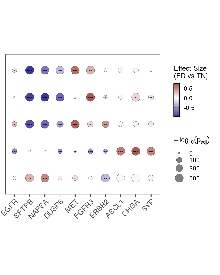
## Fig 6C — TN-vs-PD effect-size bubble heatmap
```{r bubble-heatmap-horizontal, fig.width = 4, fig.height = 5}
# Gene order is this vector, not a dendrogram. NKX2-1 is absent because the published
# panel does not show it -- it was dropped when the figure was assembled.
genes_of_int <- c(
  "EGFR", "SFTPB", "NAPSA",          # Alveolar/LUAD
  "DUSP6", "MET", "FGFR3", "ERBB2",
  "ASCL1", "CHGA", "SYP"
)
stopifnot(all(genes_of_int %in% p_val_df$feature))

bubble_df <- p_val_df %>%
  filter(feature %in% genes_of_int) %>%
  mutate(
    feature = factor(feature, levels = genes_of_int),
    patient_id = factor(patient_id, levels = rev(patients)),
    neglog10_padj = -log10(pmax(p.adj, 1e-300))
  )

p_bubble_h <- ggplot(bubble_df, aes(x = feature, y = patient_id)) +
  geom_point(aes(size = neglog10_padj, fill = wilcox_r), shape = 21, color = "grey20", stroke = 0.15) +
  geom_text(
    data = bubble_df[bubble_df$wilcox_r_label != "ns", ],
    aes(label = wilcox_r_label), size = 2, na.rm = TRUE,
    position = position_nudge(y = -0.05)
  ) +
  scale_fill_gradient2(
    low = scales::muted("blue"), mid = "white", high = scales::muted("red"),
    midpoint = 0, name = "Effect Size\n(PD vs TN)"
  ) +
  # p.adj is Bonferroni across the five patients within each gene, not an FDR, so the
  # key reads p_adj and matches the 6D y-axis.
  scale_size_continuous(name = expression(-log[10](p[adj])), range = c(1, 5)) +
  scale_x_discrete() +
  labs(x = NULL, y = NULL) +
  theme_few() +
  theme(
    axis.text.y = element_blank(),
    axis.ticks.y = element_blank(),
    panel.grid = element_blank(),
    legend.position = "right",
    legend.title = element_text(size = 9),
    legend.text = element_text(size = 8),
    plot.margin = margin(25, 2.5, 25, 2.5, unit = "mm")
  ) +
  guides(
    fill = guide_colorbar(
      keywidth = 0.5, keyheight = 3,
      ticks.colour = "black", frame.colour = "black"
    ),
    size = guide_legend(keywidth = 0.5, keyheight = 0.5, override.aes = list(fill = "grey50")),
    x = guide_axis(angle = 45)
  )

ggsave(p_bubble_h,
  filename = here("plots", "xenium", "wilcox_feature_bubble_heatmap_horizontal.pdf"),
  width = 4, height = 5
)
p_bubble_h
```
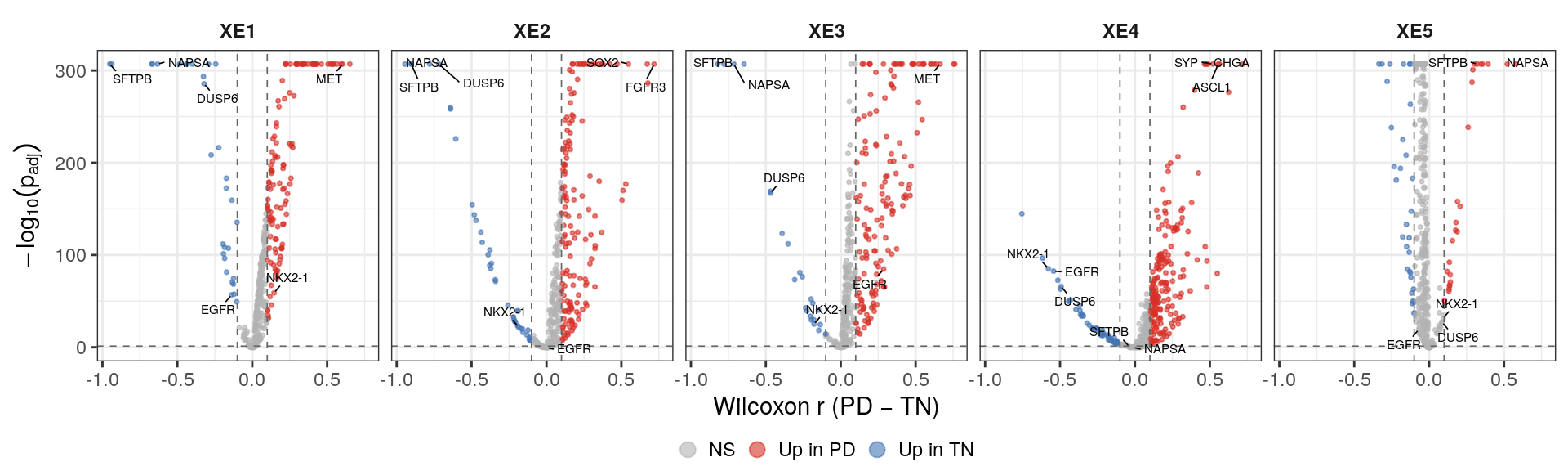
## Fig 6D — per-patient volcano
```{r, fig.width = 10, fig.height = 3}
genes_to_label <- c("EGFR", "NKX2-1", "DUSP6", "SFTPB", "NAPSA")
genes_to_label_by_patient <- list(
  XE1 = c("MET"),
  XE2 = c("FGFR3", "SOX2"),
  XE3 = c("MET"),
  XE4 = c("CHGA", "ASCL1", "SYP"),
  XE5 = c()
)
padj_cutoff <- 0.05
wilcox_r_cutoff <- 0.1

# Cap infinite -log10(p.adj) at just above the observed max
max_finite_neglog10 <- max(-log10(p_val_df$p.adj[is.finite(-log10(p_val_df$p.adj))]),
                           na.rm = TRUE)

volcano_df <- p_val_df %>%
  mutate(
    neg_log10_padj = pmin(-log10(p.adj), max_finite_neglog10 * 1.05),
    sig_direction_wr = case_when(
      p.adj < padj_cutoff & wilcox_r > wilcox_r_cutoff ~ "Up in PD",
      p.adj < padj_cutoff & wilcox_r < -wilcox_r_cutoff ~ "Up in TN",
      TRUE ~ "NS"
    )
  )

build_label_df <- function(df, effect_col, sig_col, n_top, global_genes, per_patient_genes) {
  per_pt_df <- imap_dfr(per_patient_genes, function(genes, pid) {
    if (length(genes) == 0) return(NULL)
    df %>% filter(patient_id == pid, feature %in% genes)
  })

  df %>%
    filter(.data[[sig_col]] != "NS") %>%
    group_by(patient_id, .data[[sig_col]]) %>%
    arrange(p.adj, desc(abs(.data[[effect_col]]))) %>%
    slice_head(n = n_top) %>%
    ungroup() %>%
    bind_rows(
      df %>% filter(feature %in% global_genes),
      per_pt_df
    ) %>%
    distinct(feature, patient_id, .keep_all = TRUE)
}

plot_volcano <- function(df, label_data, x_var, sig_col, x_cutoff) {
  ggplot(df, aes(x = .data[[x_var]], y = neg_log10_padj)) +
    geom_point(aes(color = .data[[sig_col]]), size = 0.6, alpha = 0.6) +
    scale_color_manual(
      values = c("Up in PD" = "#D73027", "Up in TN" = "#4575B4", "NS" = "grey70"),
      name = "Direction"
    ) +
    geom_hline(yintercept = -log10(padj_cutoff), linetype = "dashed",
               color = "grey40", linewidth = 0.3) +
    geom_vline(xintercept = c(-x_cutoff, x_cutoff), linetype = "dashed",
               color = "grey40", linewidth = 0.3) +
    ggrepel::geom_text_repel(
      data = label_data,
      aes(label = feature),
      size = 2, max.overlaps = Inf,
      min.segment.length = 0, force = 5, force_pull = 0.1,
      segment.size = 0.3, segment.color = "black",
      seed = 42
    ) +
    facet_wrap(~patient_id, nrow = 1) +
    labs(y = expression(-log[10](p[adj])),
         x = "Wilcoxon r (PD − TN)") +
    theme_bw(base_size = 11) +
    theme(
      strip.background = element_blank(),
      strip.text = element_text(face = "bold"),
      legend.position = "bottom",
      legend.margin = margin(t = -2, unit = "pt"),
      legend.spacing.x = unit(2, "pt"),
      legend.spacing.y = unit(1, "pt"),
      legend.key.size = unit(8, "pt")
    )
}

label_df_wr <- build_label_df(
  volcano_df, "wilcox_r", "sig_direction_wr",
  0, genes_to_label, genes_to_label_by_patient
)

p_volcano_wr <- plot_volcano(
  volcano_df, label_df_wr,
  x_var = "wilcox_r", sig_col = "sig_direction_wr", x_cutoff = wilcox_r_cutoff
) +
  guides(color = guide_legend(title = NULL, override.aes = list(size = 3)))

ggsave(p_volcano_wr, filename = here("plots", "xenium", "patient_volcano.pdf"),
       width = 10, height = 3)
p_volcano_wr
```
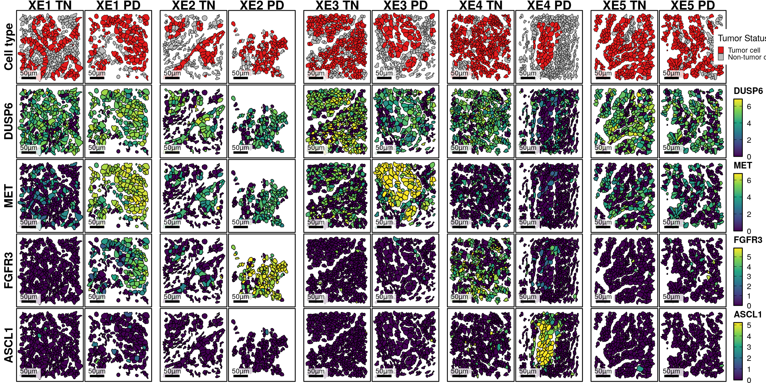
## Fig 6E — spatial marker maps
```{r}
pl_obj <- srt[, !is.na(srt$cell_type_coarse) & srt$cell_id %in% colnames(srt)[srt$in_fov]] %>%
  UpdateSeuratObject()
```
```{r, fig.width=10, fig.height=8}
axis_expand <- 0
# Fixed limit padding per side, in plot coordinates
axis_limit_pad <- 15

get_padded_limits <- function(fov_name) {
  list(
    x = crops_spec[[fov_name]]$x + c(-axis_limit_pad, axis_limit_pad),
    y = crops_spec[[fov_name]]$y + c(-axis_limit_pad, axis_limit_pad)
  )
}

pl_leg_tum <- ggplot(data.frame(tumor_cell = c("Tumor cell", "Non-tumor cell")), aes(x = as.factor(1), y = tumor_cell)) +
  geom_tile(aes(fill = tumor_cell), color = "black") +
  scale_fill_manual(name = "Tumor Status", values = c("Tumor cell" = "#e31a1c", "Non-tumor cell" = "grey"),
                    breaks = c("Tumor cell", "Non-tumor cell")) +
  guides(fill = guide_legend(keywidth = 0.5, keyheight = 0.5))
pl_leg_tum <- ggpubr::get_legend(pl_leg_tum)
pl_leg_tum <- ggpubr::as_ggplot(pl_leg_tum)

# Tumor vs non-tumor, the top row of the Fig 6E grid
pl_obj$tumor_cell <- ifelse(pl_obj$cell_type_coarse == "Tumor", "Tumor cell", "Non-tumor cell")
pl_tum <- ImageDimPlot(pl_obj,
                   fov = names(crops_spec),
                   group.by = c("tumor_cell"),
                   axes = TRUE,
                   border.color = "black",
                   border.size = 0.2,
                   crop = T,
                   cols = c("Tumor cell" = "#e31a1c", "Non-tumor cell" = "grey"),
                   coord.fixed = T,
                   dark.background = F,
                   combine = F)
pl_tum <- map2(pl_tum, names(crops_spec), function(p, fov_name) {
  lims <- get_padded_limits(fov_name)
  p +
    scale_x_continuous(
      limits = lims$x,
      expand = expansion(mult = c(axis_expand, axis_expand))
    ) +
    scale_y_continuous(
      limits = lims$y,
      expand = expansion(mult = c(axis_expand, axis_expand))
    )
})
names(pl_tum) <- names(crops_spec)
```
```{r}
# The four feature rows of Fig 6E, under the tumor/non-tumor row.
ft_list <- c("DUSP6", "MET", "FGFR3", "ASCL1")

# Per-feature q99, computed over the whole object so the colour scale is comparable
# across FOVs.
cli::cli_h3("Computing global q99 quantiles for {length(ft_list)} features")

feature_matrix <- FetchData(pl_obj, vars = ft_list)
feature_quantiles <- setNames(
  apply(feature_matrix, 2, function(x) {
    q99 <- quantile(x, probs = 0.99, na.rm = TRUE)
    if (q99 == 0) max(x, na.rm = TRUE) else q99
  }),
  ft_list
)
rm(feature_matrix)

fov_names <- names(crops_spec)

cli::cli_h3("Plotting {length(ft_list)} features across {length(fov_names)} FOVs")

pl_feats_by_feature <- setNames(vector("list", length(ft_list)), ft_list)

for (i in seq_along(ft_list)) {
  ft <- ft_list[[i]]
  cli::cli_progress_step("({i}/{length(ft_list)}) {ft}")
  plots <- ImageFeaturePlot(
    pl_obj,
    features        = ft,
    border.color    = "black",
    fov             = fov_names,
    scale           = "all",
    axes            = TRUE,
    crop            = TRUE,
    dark.background = FALSE,
    coord.fixed     = TRUE,
    combine         = FALSE
  ) %>%
    map2(fov_names, .f = function(p, fov_name) {
      lims <- get_padded_limits(fov_name)
      p +
        scale_x_continuous(
          limits = lims$x,
          expand = expansion(mult = c(axis_expand, axis_expand))
        ) +
        scale_y_continuous(
          limits = lims$y,
          expand = expansion(mult = c(axis_expand, axis_expand))
        ) +
        scale_fill_viridis_c(option = "viridis",
                             limits = c(0, feature_quantiles[[ft]]),
                             oob = scales::squish) +
        theme_classic() +
        theme(axis.line = element_blank(),
              panel.border = element_rect(fill = NA, linewidth = 0.25)) +
        guides(fill = guide_colorbar(keywidth = 0.75,
                                     keyheight = 5,
                                     frame.colour = "black",
                                     ticks.colour = "black"))
    })
  pl_feats_by_feature[[ft]] <- setNames(plots, fov_names)
}

# Reshape into nested: fov -> feature -> plot
pl_feats <- setNames(
  lapply(fov_names, function(fov_name) {
    setNames(lapply(pl_feats_by_feature, `[[`, fov_name), ft_list)
  }),
  fov_names
)
```
```{r, fig.width = 22/1.2, fig.height = 60/1.2}
# Grid: rows = cell types + mutations + each feature; columns = FOVs paired TN | PD per
# patient under a shared patient title

# Coordinates are in μm; scale bar length in μm
SCALE_BAR_UM <- 50

# yr[1] = small y = visual bottom; yr[2] = large y = visual top (no y reversal in ImageFeaturePlot)
add_scale_bar <- function(p, spec) {
  xr   <- spec$x
  yr   <- spec$y
  xpad <- diff(xr) * 0.01   # horizontal offset from left edge (increase → moves bar right)
  ypad <- diff(yr) * 0.01   # vertical offset from bottom edge (increase → moves bar up)
  x0   <- xr[1] + xpad      # bar left endpoint
  x1   <- x0 + SCALE_BAR_UM # bar right endpoint (bar length in μm)
  ybar <- yr[1] + ypad       # y position of the bar line
  ylab <- ybar + diff(yr) * 0.08  # y position of label text (increase multiplier → more gap between bar and text)

  box_xpad <- diff(xr) * 0.08  # extra horizontal padding around bar (increase → wider box)
  box_ypad <- diff(yr) * 0.05  # padding below the bar (increase → taller box below)
  box_x0   <- x0 - box_xpad    # box left edge
  box_x1   <- x1 + box_xpad    # box right edge
  box_y0   <- ybar - box_ypad   # box bottom edge
  box_y1   <- ylab + diff(yr) * 0.04  # box top edge (increase → taller box above label)

  p +
    annotate("rect", xmin = box_x0, xmax = box_x1, ymin = box_y0, ymax = box_y1,
             fill = "white", color = NA, alpha = 0.8) +  # semi-transparent white background
    annotate("segment", x = x0, xend = x1, y = ybar, yend = ybar,
             color = "black", linewidth = 1.4) +  # the scale bar line (linewidth controls thickness)
    annotate("text", x = (x0 + x1) / 2, y = ylab,
             label = paste0(SCALE_BAR_UM, "µm"),
             color = "black", size = 3, hjust = 0.5)  # label text (size controls font size)
}

polish_plot <- function(p, spec) {
  p_themed <- p +
    theme_classic() +
    theme(
      plot.title   = element_blank(),
      axis.line    = element_blank(),
      axis.title   = element_blank(),
      axis.text    = element_blank(),
      axis.ticks   = element_blank(),
      panel.border = element_rect(fill = NA, linewidth = 0.5)
    )
  add_scale_bar(p_themed, spec)
}

strip_legend <- function(p) p + theme(legend.position = "none")
keep_legend  <- function(p) p + theme(
  legend.position      = "right",
  legend.justification = "left",
  legend.title.align   = 0,
  legend.key.height    = unit(0.55, "cm"),
  legend.key.width     = unit(0.4, "cm"),
  legend.text          = element_text(size = 10),
  legend.background = element_blank(),
  plot.background = element_blank(),
  legend.title         = element_text(size = 11, face = "bold")
)

make_row_label <- function(label) {
  ggplot() +
    annotate("text", x = 0.5, y = 0.5,
             label = label, angle = 90,
             size = 5, fontface = "bold", hjust = 0.5, vjust = 0.5) +
    theme_void()
}

# Build one row: [label | TN PD spacer TN PD spacer ... TN PD | legend]
make_row <- function(plot_by_fov, label) {
  plots <- lapply(patients, function(pt) {
    tn_name <- paste0(pt, "_TN_crop")
    pd_name <- paste0(pt, "_PD_crop")
    list(
      polish_plot(plot_by_fov[[tn_name]], crops_spec[[tn_name]]),
      polish_plot(plot_by_fov[[pd_name]], crops_spec[[pd_name]])
    )
  })
  last_plot <- plots[[length(plots)]][[2]]
  leg <- cowplot::get_legend(keep_legend(last_plot))
  panels <- list()
  for (i in seq_along(plots)) {
    panels <- c(panels, lapply(plots[[i]], strip_legend))
    if (i < length(plots)) panels <- c(panels, list(plot_spacer()))
  }
  c(list(make_row_label(label)), panels, list(cowplot::ggdraw(leg)))
}

pl_leg <- pl_leg_tum
make_row_ct <- function(plot_by_fov, label) {
  plots <- lapply(patients, function(pt) {
    tn_name <- paste0(pt, "_TN_crop")
    pd_name <- paste0(pt, "_PD_crop")
    list(
      polish_plot(plot_by_fov[[tn_name]], crops_spec[[tn_name]]),
      polish_plot(plot_by_fov[[pd_name]], crops_spec[[pd_name]])
    )
  })
  panels <- list()
  for (i in seq_along(plots)) {
    panels <- c(panels, lapply(plots[[i]], strip_legend))
    if (i < length(plots)) panels <- c(panels, list(plot_spacer()))
  }
  c(list(make_row_label(label)), panels, list(pl_leg))
}

col_header_plots <- c(
  list(plot_spacer()),  # blank over row-label column
  unlist(lapply(seq_along(patients), function(i) {
    pt <- patients[i]
    hdrs <- lapply(c(paste0(pt, " TN"), paste0(pt, " PD")), function(lbl) {
      ggplot() +
        annotate("text", x = 0.5, y = 0.5, label = lbl, size = 5.5, fontface = "bold") +
        theme_void()
    })
    if (i < length(patients)) c(hdrs, list(plot_spacer())) else hdrs
  }), recursive = FALSE),
  list(plot_spacer())  # blank over legend column
)

row_specs <- c(
  list(cell_type = pl_tum),
  setNames(lapply(ft_list, function(ft) lapply(pl_feats, `[[`, ft)), ft_list)
)

# ncols = 1 (row label) + patients * 2 (FOV panels) + (patients-1) spacers + 1 (legend)
n_spacers <- length(patients) - 1
ncols <- 1 + length(patients) * 2 + n_spacers + 1

# Widths: row-label, then per patient (1, 1) with spacer between pairs, then legend
panel_widths <- unlist(lapply(seq_along(patients), function(i) {
  if (i < length(patients)) c(1, 1, 0.08) else c(1, 1)
}))

pl_grid <- wrap_plots(
  c(
    col_header_plots,
    unlist(
      lapply(names(row_specs), function(nm) {
        if (nm == "cell_type") make_row_ct(row_specs[[nm]], "Cell type")
        else                   make_row(row_specs[[nm]], nm)
      }),
      recursive = FALSE
    )
  ),
  ncol   = ncols,
  byrow  = TRUE,
  widths  = c(0.2, panel_widths, 0.55),
  heights = c(0.1, rep(1, length(row_specs)))  # header row shorter
)

pcomb <- pl_grid +
  plot_annotation(
    theme = theme(plot.title = element_text(size = 14, face = "bold"))
  ) &
  theme(plot.margin = margin(1, 1, 1, 1, "pt"),
        legend.background = element_blank(),
        strip.clip = "off",
        legend.box.background = element_blank(),
        legend.justification = "left",
        legend.key = element_blank(),
        panel.background = element_blank(),
        plot.background = element_blank()) &
  coord_cartesian(clip = "off")
```
```{r, fig.width = 16/1.2, fig.height = 8/1.2}
ggsave(pcomb, filename = here("plots", "xenium", "select_features_spatial_plot.pdf"), width = 16/1.2, height = 8/1.2)
pcomb
```
```{r release-spatial-plots}
#| include: false
# Each ImageFeaturePlot copies the coordinates of every cell it draws, so the FOV plot lists
# are the largest thing in the session. The grid above is their last use.
rm(list = intersect(c("pl_feats", "pl_feats_by_feature", "pl_obj", "pl_grid",
"feature_quantiles", "row_specs"), ls()))
invisible(gc(full = TRUE))
```
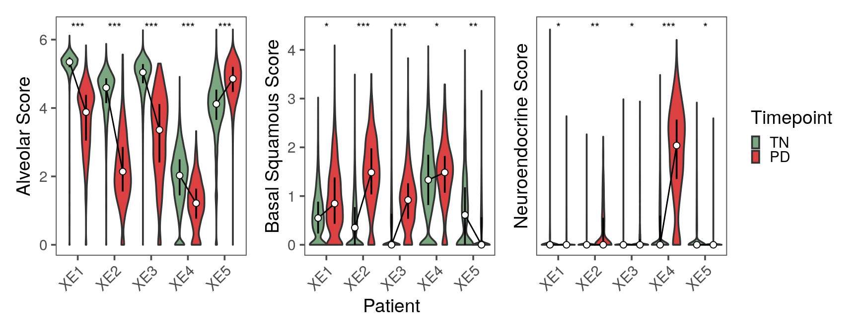
## Fig 6F — paired pathway-score violins
```{r}
paths <- paste0(names(lung_lineage_genes), "_score")
df_paths <- FetchData(srt[, srt$is_tumor_cell],
  vars = c("patient_id", "timepoint", "cell_type_coarse", paths)
)
df_paths$timepoint <- fct_relevel(df_paths$timepoint, "TN", "PD")

p_val_df_paths <- fast_wilcox(df_paths, paths) %>%
  group_by(feature) %>%
  mutate(
    p = pmax(p, .Machine$double.xmin),
    p.adj = p.adjust(p, method = "bonferroni")
  ) %>%
  ungroup() %>%
  mutate(
    p.adj.signif = case_when(
      is.na(p.adj) ~ NA_character_,
      p.adj < 1e-4 ~ "****", p.adj < 1e-3 ~ "***",
      p.adj < 1e-2 ~ "**",   p.adj < 5e-2 ~ "*",
      TRUE ~ "ns"
    ),
    wilcox_r_mag = case_when(
      is.na(wilcox_r) ~ NA_character_,
      abs(wilcox_r) < 0.1 ~ "negligible", abs(wilcox_r) < 0.3 ~ "small",
      abs(wilcox_r) < 0.5 ~ "moderate",   TRUE ~ "large"
    )
  ) %>%
  arrange(feature, patient_id)

p_val_df_paths$wilcox_r <- -p_val_df_paths$wilcox_r
p_val_df_paths$wilcox_r_label <- case_when(
  is.na(p_val_df_paths$wilcox_r) ~ NA_character_,
  abs(p_val_df_paths$wilcox_r) < 0.1 ~ "ns", abs(p_val_df_paths$wilcox_r) < 0.3 ~ "*",
  abs(p_val_df_paths$wilcox_r) < 0.5 ~ "**", TRUE ~ "***"
)

p_val_df_paths$pct_diff <- p_val_df_paths$pct_PD - p_val_df_paths$pct_TN

p_val_df_paths <- p_val_df_paths %>%
  group_by(feature) %>%
  mutate(gene_max = max(max_tn, max_pd)) %>%
  ungroup()
```
```{r}
pls_paths <- map(paths, .f = function(ft) {
  p <- df_paths %>%
    ggplot(aes(x = patient_id, y = .data[[ft]])) +
    geom_violin(
      scale = "width", show.legend = T, aes(fill = timepoint),
      position = position_dodge(width = 0.9)
    ) +
    geom_segment(
      data = df_paths %>%
        group_by(patient_id, timepoint) %>%
        summarise(y = median(.data[[ft]]), .groups = "drop") %>%
        pivot_wider(names_from = timepoint, values_from = y) %>%
        mutate(x_num = as.numeric(factor(patient_id, levels = levels(factor(df_paths$patient_id))))),
      aes(
        x = x_num - 0.9 / 4, xend = x_num + 0.9 / 4,
        y = TN, yend = PD
      ), linetype = "solid",
      inherit.aes = FALSE,
        linewidth = 0.5
    ) +
    geom_pointrange(aes(group = timepoint),
      pch = 21, fill = "white", stroke = 0.5,
      stat = "summary", size = 0.5, position = position_dodge(width = 0.9),
      fun.min = function(z) {
        quantile(z, 0.25)
      },
      fun.max = function(z) {
        quantile(z, 0.75)
      },
      fun = median
    ) +
    ggprism::add_pvalue(
      data = p_val_df_paths[p_val_df_paths$feature == ft, ],
      y.position = max(p_val_df_paths$gene_max[p_val_df_paths$feature == ft], na.rm = TRUE) * 1.01,
      label = "{wilcox_r_label}", tip.length = 0.1, x = "patient_id"
    ) +
    scale_fill_manual(values = colors$time_point) +
    theme_few(base_size = 14) +
    theme(
      axis.text.x = element_text(angle = 45, hjust = 1),
      strip.background = element_rect(fill = NA, color = "black")
    ) +
    labs(x = "Patient", fill = "Timepoint", y = str_to_title(gsub("_", " ", ft)))
  p
})
names(pls_paths) <- paths
```
```{r, fig.width = 9, fig.height = 3.5}
pcomb <- pls_paths$alveolar_score + pls_paths$basal_squamous_score + pls_paths$neuroendocrine_score +
  plot_layout(guides = "collect", axes = "collect", ncol = 3) &
  theme(legend.position = "right") &
  guides(fill = guide_legend(keywidth = 0.5, keyheight = 0.5))
ggsave(pcomb, filename = here("plots", "xenium", "wilcox_pathway_score_plots.pdf"), width = 9, height = 3.5)
pcomb
```
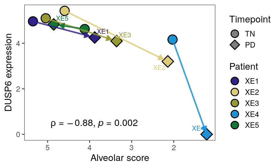
## Fig 6G — DUSP6 vs alveolar score arrow plot
```{r, fig.width = 5, fig.height = 3}
df <- FetchData(srt, vars = c("DUSP6", "alveolar_score", "patient_id", "timepoint", "cell_type_coarse", "is_tumor_cell")) %>%
  filter(is_tumor_cell)

df_med <- df %>%
  group_by(patient_id, timepoint) %>%
  summarize(DUSP6 = median(DUSP6), alveolar = median(alveolar_score), .groups = "drop")

df_seg <- df_med %>%
  group_by(patient_id) %>%
  summarize(
    x = alveolar[timepoint == "TN"][1],
    xend = alveolar[timepoint == "PD"][1],
    y = DUSP6[timepoint == "TN"][1],
    yend = DUSP6[timepoint == "PD"][1],
    .groups = "drop"
  ) %>%
  filter(!is.na(x), !is.na(xend), !is.na(y), !is.na(yend))

p <- df_med %>%
  ggplot(aes(x = alveolar, y = DUSP6)) +
  geom_point(aes(fill = patient_id, shape = timepoint), size = 5, stroke = 0.85) +
  ggarchery::geom_arrowsegment(data = df_seg,
               aes(x = x, xend = xend, y = y, yend = yend, color = patient_id, fill = patient_id),
               arrows = arrow(length = unit(0.22, "cm"), type = "closed"),
               linewidth = 0.9,
               alpha = 0.85,
               show.legend = FALSE,
               position = ggarchery::position_attractsegment(start_shave = 0,
                                                  end_shave = 0.15,
                                                  type_shave = "distance")) +
  ggrepel::geom_text_repel(
    data = df_med %>% filter(timepoint == "PD"),
    aes(label = patient_id, color = patient_id),
    size = 3,
    box.padding = 0.25,
    point.padding = 0.15,
    min.segment.length = Inf,
    show.legend = FALSE,
    seed = 42
  ) +
  scale_color_manual(values = colors$xe_pts) +
  scale_fill_manual(values = colors$xe_pts) +
  scale_shape_manual(values = c("TN" = 21,
                                "PD" = 23),
                     breaks = c("TN", "PD")) +
  scale_x_reverse() +
  ggpubr::stat_cor(method = "spearman", cor.coef.name = "rho", label.x.npc = 0.1, label.y.npc = 0.1) +
  theme_few() +
  guides(
    shape = guide_legend(order = 1, override.aes = list(fill = "grey50", size = 4)),
    fill = guide_legend(order = 2, override.aes = list(shape = 21, size = 4, alpha = 1))
  ) +
  theme(
    legend.key.height = unit(0.5, "cm"),
    legend.key.width = unit(0.5, "cm"),
    legend.spacing.y = unit(0.1, "cm")
  ) +
  labs(x = "Alveolar score", y = "DUSP6 expression",
       fill = "Patient", shape = "Timepoint")
ggsave(p, filename = here("plots", "xenium", "DUSP6_vs_alveolar_score.pdf"), width = 5, height = 3)
p
```
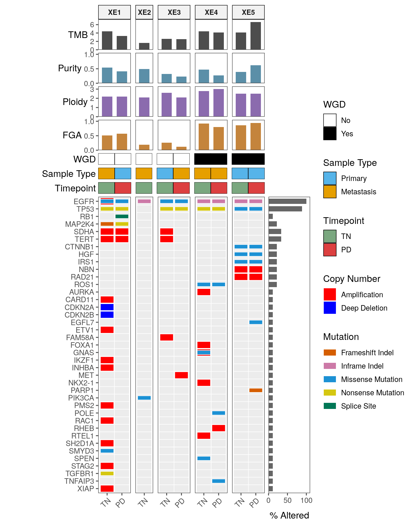
## Fig S11A — IMPACT oncoprint, Xenium-matched samples
```{r oncoplot-data}
# Nine IMPACT-profiled samples, ordered TN then PD within patient.
xe_sample_order <- xe_meta %>%
  filter(has_impact) %>%
  arrange(patient_id, timepoint) %>%
  pull(sample_id)

xe_sample_meta <- xe_meta %>%
  filter(has_impact) %>%
  left_join(facets$samples %>% dplyr::select(sample_id, sample_type), by = "sample_id") %>%
  transmute(
    sample_id = factor(sample_id, levels = xe_sample_order),
    patient_id,
    xe_timepoint = timepoint,
    cvr_tmb_score = facets_tmb,
    purity = facets_purity,
    ploidy = facets_ploidy,
    fga = facets_fga,
    wgd = facets_wgd,
    sample_type = fct_relevel(sample_type, "Primary", "Metastasis")
  ) %>%
  arrange(sample_id)
stopifnot(nrow(xe_sample_meta) == 9L, !any(is.na(xe_sample_meta$sample_type)))

xe_onco_mut <- xe_muts %>%
  mutate(
    sample_id = factor(sample_id, levels = xe_sample_order),
    patient_id = factor(patient_id, levels = patients)
  )
stopifnot(!any(is.na(xe_onco_mut$sample_id)))

# Gene frequency over the nine samples; dplyr::count() returns genes alphabetically, so
# the descending-frequency sort is deterministic within ties.
xe_gene_freq <- xe_onco_mut %>%
  distinct(sample_id, gene) %>%
  dplyr::count(gene, name = "n_samples") %>%
  mutate(freq = n_samples / length(xe_sample_order)) %>%
  arrange(desc(freq))

# EGFR / TP53 / RB1 / FGFR3 / MAP2K4 are pinned to the top; the rest sort by frequency.
# FGFR3 is not altered in any Xenium-matched sample, so intersect() drops it.
pinned <- c("EGFR", "TP53", "RB1", "FGFR3", "MAP2K4")
xe_gene_order <- c(
  intersect(pinned, xe_gene_freq$gene),
  xe_gene_freq %>% filter(!gene %in% pinned) %>% arrange(desc(freq)) %>% pull(gene)
)
```
```{r oncoplot-layers}
theme_onco_strip <- theme_few() +
  theme(
    axis.text.x = element_blank(),
    axis.ticks.x = element_blank(),
    axis.title.x = element_blank(),
    axis.title.y = element_text(angle = 0, vjust = 0.5, hjust = 1),
    strip.background = element_rect(fill = "grey95", color = "black"),
    strip.text = element_text(size = 9, face = "bold"),
    plot.margin = margin(1, 2, 3, 2, unit = "pt")
  )

theme_onco_tile <- theme_onco_strip +
  theme(
    axis.text.y = element_blank(),
    axis.ticks.y = element_blank(),
    panel.border = element_blank()
  )

scale_tile_x <- scale_x_discrete(expand = c(0, 0))
scale_tile_y <- scale_y_discrete(expand = c(0, 0))
shared_facet <- facet_grid(. ~ patient_id, scales = "free_x", space = "free_x")
stype_pal <- c("Primary" = "#56B4E9", "Metastasis" = "#E69F00")

# The three mutation layers use different tile heights so an SSM stacked on a CNA stays
# legible. "Other" is kept in both the filter and the palette so a class that falls through
# the upstream case_when() still renders rather than dropping out of every layer; unused
# palette names do not reach the legend.
CNA_CLASSES <- c("Amplification", "Deep Deletion")
SSM_CLASSES <- c(
  "Missense Mutation", "Nonsense Mutation", "Frameshift Indel",
  "Inframe Indel", "Splice Site", "Other"
)
FUSION_CLASSES <- c("RNA Fusion", "Structural Variant")
stopifnot(all(xe_onco_mut$mut_class %in% c(CNA_CLASSES, SSM_CLASSES, FUSION_CLASSES)))

xe_cna <- xe_onco_mut %>% filter(mut_class %in% CNA_CLASSES)
xe_ssm <- xe_onco_mut %>% filter(mut_class %in% SSM_CLASSES)
xe_fusion <- xe_onco_mut %>% filter(mut_class %in% FUSION_CLASSES)

xe_grid_df <- expand.grid(
  sample_id = xe_sample_order,
  gene = xe_gene_order,
  stringsAsFactors = FALSE
) %>%
  left_join(xe_sample_meta %>% transmute(sample_id = as.character(sample_id), patient_id),
    by = "sample_id"
  ) %>%
  mutate(sample_id = factor(sample_id, levels = xe_sample_order))

# Legend key glyphs matching the tile geometry (full-height CNA, half-height SSM).
draw_key_full_rect <- function(data, params, size) {
  grid::rectGrob(
    width = grid::unit(0.9, "snpc"), height = grid::unit(0.9, "snpc"),
    gp = grid::gpar(col = NA, fill = scales::alpha(
      if (is.null(data$fill)) "grey20" else data$fill,
      if (is.null(data$alpha)) 1 else data$alpha
    ))
  )
}

draw_key_short_rect <- function(data, params, size) {
  grid::rectGrob(
    width = grid::unit(0.9, "snpc"), height = grid::unit(0.45, "snpc"),
    gp = grid::gpar(col = NA, fill = scales::alpha(
      if (is.null(data$fill)) "grey20" else data$fill,
      if (is.null(data$alpha)) 1 else data$alpha
    ))
  )
}

xp_tmb <- ggplot(xe_sample_meta, aes(x = sample_id, y = cvr_tmb_score)) +
  geom_col(fill = "grey30", width = 0.7) +
  scale_y_continuous(expand = expansion(mult = c(0, 0.1))) +
  shared_facet +
  theme_onco_strip +
  labs(y = "TMB")

xp_purity <- ggplot(xe_sample_meta, aes(x = sample_id, y = purity)) +
  geom_col(fill = "#5B8FA8", width = 0.7) +
  scale_y_continuous(limits = c(0, 1), breaks = c(0, 0.5, 1), expand = expansion(mult = c(0, 0.05))) +
  shared_facet +
  theme_onco_strip +
  labs(y = "Purity")

xp_ploidy <- ggplot(xe_sample_meta, aes(x = sample_id, y = ploidy)) +
  geom_col(fill = "#8B6BAE", width = 0.7) +
  scale_y_continuous(expand = expansion(mult = c(0, 0.1))) +
  shared_facet +
  theme_onco_strip +
  labs(y = "Ploidy")

xp_fga <- ggplot(xe_sample_meta, aes(x = sample_id, y = fga)) +
  geom_col(fill = "#C4843C", width = 0.7) +
  scale_y_continuous(limits = c(0, 1), breaks = c(0, 0.5, 1), expand = expansion(mult = c(0, 0.05))) +
  shared_facet +
  theme_onco_strip +
  labs(y = "FGA")

xp_wgd <- ggplot(xe_sample_meta, aes(x = sample_id, y = "WGD")) +
  geom_tile(aes(fill = as.character(wgd)), color = "black", linewidth = 0.3) +
  scale_fill_manual(
    name = "WGD", values = c("TRUE" = "black", "FALSE" = "white"),
    labels = c("TRUE" = "Yes", "FALSE" = "No"), na.value = "grey80"
  ) +
  shared_facet +
  theme_onco_tile +
  scale_tile_x +
  scale_tile_y +
  labs(y = "WGD") +
  theme(axis.title.y = element_text(angle = 0, vjust = 0.5))

xp_stype <- ggplot(xe_sample_meta, aes(x = sample_id, y = "Type")) +
  geom_tile(aes(fill = sample_type), color = "black", linewidth = 0.3) +
  scale_fill_manual(name = "Sample Type", values = stype_pal, na.value = "grey80") +
  shared_facet +
  theme_onco_tile +
  scale_tile_x +
  scale_tile_y +
  labs(y = "Sample Type") +
  theme(axis.title.y = element_text(angle = 0, vjust = 0.5))

xp_tp <- ggplot(xe_sample_meta, aes(x = sample_id, y = "Timepoint")) +
  geom_tile(aes(fill = xe_timepoint), color = "black", linewidth = 0.3) +
  scale_fill_manual(name = "Timepoint", values = colors$time_point, na.value = "grey80") +
  shared_facet +
  theme_onco_tile +
  scale_tile_x +
  scale_tile_y +
  labs(y = "Timepoint") +
  theme(axis.title.y = element_text(angle = 0, vjust = 0.5))

xp_grid <- ggplot() +
  geom_tile(
    data = xe_grid_df, aes(x = sample_id, y = gene),
    fill = "#ECECEC", color = "white", linewidth = 0.3
  ) +
  geom_tile(
    data = xe_cna, aes(x = sample_id, y = gene, fill = mut_class),
    color = "white", linewidth = 0.3, height = 0.9, width = 0.9,
    key_glyph = draw_key_full_rect
  ) +
  scale_fill_manual(
    name = "Copy Number",
    values = c("Amplification" = "red", "Deep Deletion" = "blue"),
    guide = guide_legend(order = 1)
  ) +
  ggnewscale::new_scale_fill() +
  geom_tile(
    data = xe_ssm, aes(x = sample_id, y = gene, fill = mut_class),
    color = "white", linewidth = 0.3, height = 0.55, width = 0.9,
    key_glyph = draw_key_short_rect
  ) +
  geom_tile(
    data = xe_fusion, aes(x = sample_id, y = gene, fill = mut_class),
    color = "white", linewidth = 0.3, height = 0.9, width = 0.35,
    key_glyph = draw_key_short_rect
  ) +
  scale_fill_manual(
    name = "Mutation",
    values = c(
      "Missense Mutation" = "#1C91D4",
      "Nonsense Mutation" = "#D5C711",
      "Frameshift Indel" = "#D55E00",
      "Inframe Indel" = "#CC79A7",
      "RNA Fusion" = "#F0E442",
      "Structural Variant" = "#56B4E9",
      "Splice Site" = "#007756",
      "Other" = "#007756"
    ),
    guide = guide_legend(order = 2)
  ) +
  scale_y_discrete(limits = rev(xe_gene_order)) +
  shared_facet +
  theme_few() +
  theme(
    axis.text.x = element_text(angle = 45, hjust = 1),
    strip.background = element_rect(fill = "grey95", color = "black"),
    strip.text = element_text(size = 9, face = "bold"),
    plot.margin = margin(1, 5, 5, 5, unit = "pt"),
    panel.grid = element_blank()
  ) +
  labs(y = NULL, x = NULL) +
  scale_x_discrete(labels = setNames(
    as.character(xe_sample_meta$xe_timepoint),
    as.character(xe_sample_meta$sample_id)
  ))

xp_freq <- ggplot(xe_gene_freq, aes(x = freq * 100, y = gene)) +
  geom_col(fill = "grey40", width = 0.7) +
  scale_y_discrete(limits = rev(xe_gene_order)) +
  scale_x_continuous(expand = expansion(mult = c(0, 0.1)), breaks = c(0, 50, 100)) +
  theme_few() +
  theme(
    axis.text.y = element_blank(), axis.ticks.y = element_blank(),
    plot.margin = margin(1, 5, 5, 0, unit = "pt"), panel.grid.major.y = element_blank()
  ) +
  labs(x = "% Altered", y = NULL)
```
```{r oncoplot, fig.width = 7.5, fig.height = 9.5}
xe_n_genes <- max(length(xe_gene_order), 8)
no_strip <- theme(strip.text = element_blank(), strip.background = element_blank())

xe_design <- "
AAAAAAAA##
BBBBBBBB##
CCCCCCCC##
DDDDDDDD##
EEEEEEEE##
FFFFFFFF##
GGGGGGGG##
HHHHHHHHII
"

xe_oncoplot <-
  free(xp_tmb, type = "label", side = "l") +
  free((xp_purity + no_strip), type = "label", side = "l") +
  free((xp_ploidy + no_strip), type = "label", side = "l") +
  free((xp_fga + no_strip), type = "label", side = "l") +
  free((xp_wgd + no_strip), type = "label", side = "l") +
  free((xp_stype + no_strip), type = "label", side = "l") +
  free((xp_tp + no_strip), type = "label", side = "l") +
  (xp_grid + no_strip) +
  xp_freq +
  plot_layout(
    design = xe_design,
    heights = c(4, 4, 4, 4, 1.5, 1.5, 1.5, xe_n_genes),
    guides = "collect"
  ) &
  theme(legend.position = "right")

ggsave(xe_oncoplot,
  filename = here("plots", "xenium", "oncoplot_impact_xenium_matched.pdf"),
  width = 7.5, height = 9.5
)
xe_oncoplot
```
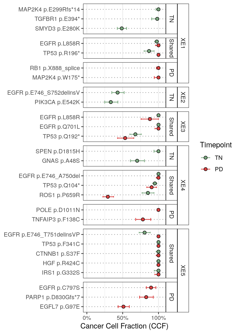
## Fig S11B — cancer cell fractions, TN vs PD
```{r ccf-data}
ccf_plot_df <- xe_muts %>%
  filter(!is.na(ccf_expected_copies)) %>%
  mutate(mut_label = paste0(gene, " ", HGVSp_Short))
stopifnot(nrow(ccf_plot_df) == 40L)

mut_status <- ccf_plot_df %>%
  distinct(patient_id, mut_label, timepoint) %>%
  group_by(patient_id, mut_label) %>%
  dplyr::summarize(
    has_TN = any(timepoint == "TN"),
    has_PD = any(timepoint == "PD"),
    .groups = "drop"
  ) %>%
  mutate(status = factor(
    case_when(has_TN & has_PD ~ "Shared", !has_TN & has_PD ~ "PD", has_TN & !has_PD ~ "TN"),
    levels = c("Shared", "PD", "TN")
  ))

ccf_plot_df <- ccf_plot_df %>%
  left_join(mut_status %>% dplyr::select(patient_id, mut_label, status),
    by = c("patient_id", "mut_label")
  ) %>%
  filter(!is.na(status)) %>%
  # PD before TN in the dodge order; the legend is re-ordered back to TN, PD by `breaks`.
  mutate(timepoint = factor(timepoint, levels = c("PD", "TN")))

# Within each patient x status block: pinned genes first, then descending CCF (the TN
# value for shared mutations, so a shared pair sorts on where it started).
ccf_plot_df <- ccf_plot_df %>%
  group_by(patient_id, status, mut_label) %>%
  mutate(
    sort_ccf = case_when(
      status == "Shared" & any(timepoint == "TN") ~ ccf_expected_copies[timepoint == "TN"][1],
      .default = max(ccf_expected_copies, na.rm = TRUE)
    ),
    is_pinned = gene %in% pinned,
    pin_rank = match(gene, pinned, nomatch = length(pinned) + 1L)
  ) %>%
  ungroup() %>%
  arrange(patient_id, status, desc(is_pinned), pin_rank, desc(sort_ccf)) %>%
  mutate(mut_label = fct_rev(fct_inorder(mut_label)))

stopifnot(all(levels(ccf_plot_df$timepoint) %in% names(colors$time_point)))
```
```{r ccf, fig.width = 5, fig.height = 7}
p_ccf <- ggplot(ccf_plot_df, aes(x = ccf_expected_copies, y = mut_label)) +
  geom_errorbar(
    aes(
      xmin = ccf_expected_copies_lower, xmax = ccf_expected_copies_upper,
      color = timepoint
    ),
    orientation = "y", width = 0.3,
    position = position_dodge(width = 0.8)
  ) +
  geom_point(
    aes(fill = timepoint),
    size = 2, pch = 21, stroke = 0.5,
    position = position_dodge(width = 0.8)
  ) +
  scale_fill_manual(values = colors$time_point, name = "Timepoint", breaks = c("TN", "PD")) +
  scale_color_manual(values = colors$time_point, name = "Timepoint", breaks = c("TN", "PD")) +
  scale_x_continuous(
    limits = c(0, 1.05), breaks = c(0, 0.5, 1),
    labels = scales::percent_format()
  ) +
  facet_nested(
    patient_id + fct_relevel(status, "TN", "Shared", "PD") ~ .,
    scales = "free_y", space = "free_y", strip = strip_nested(bleed = FALSE)
  ) +
  theme_bw() +
  theme(
    strip.background = element_rect(fill = NA),
    panel.grid.major.y = element_line(linetype = "dotted", color = "grey60")
  ) +
  labs(x = "Cancer Cell Fraction (CCF)", y = NULL)

ggsave(p_ccf,
  filename = here("plots", "xenium", "ccf_comparison_by_status.pdf"),
  width = 5, height = 7
)
p_ccf
```
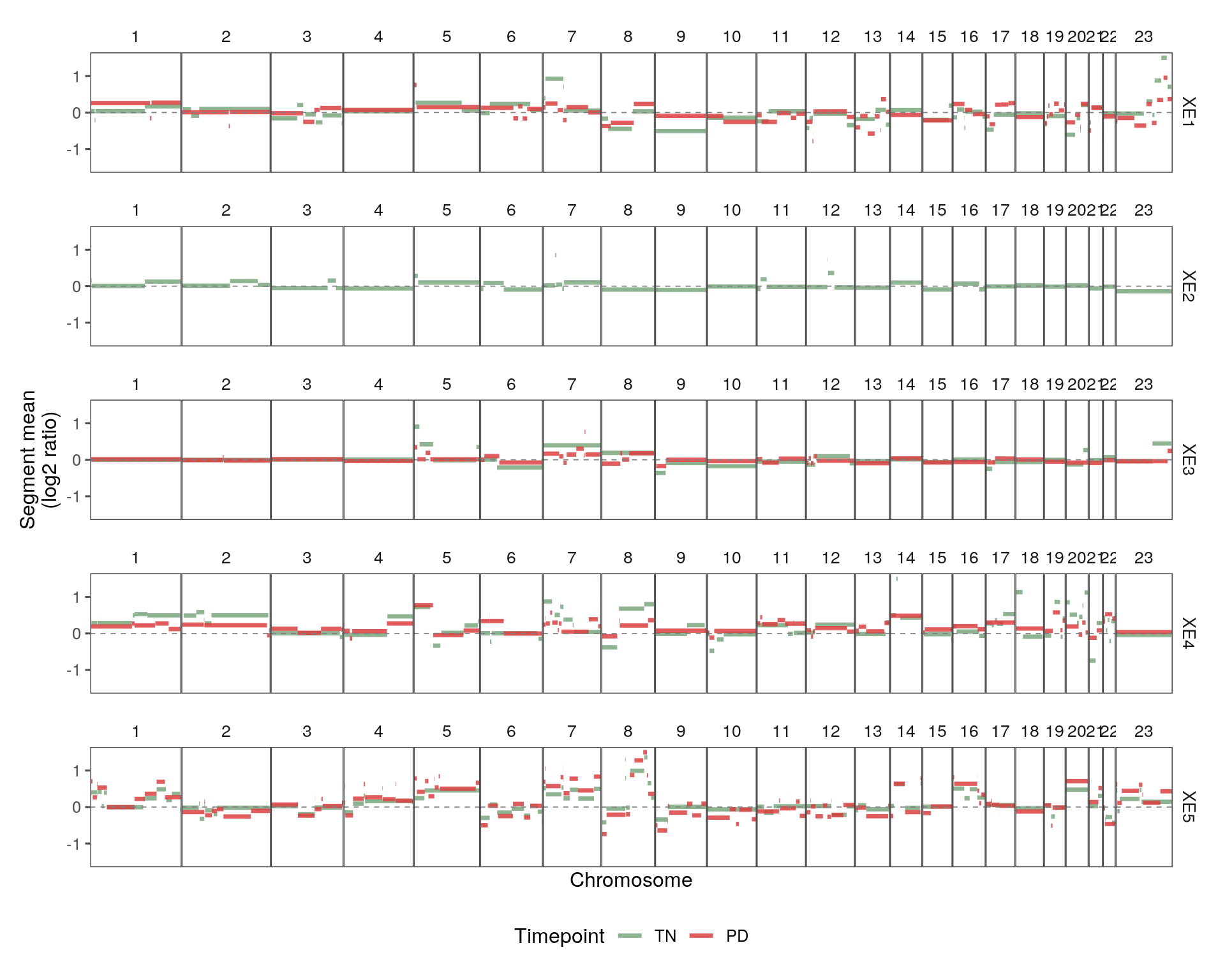
## Fig S11C — copy number profiles, TN vs PD
```{r cn-profiles, fig.width = 10, fig.height = 8}
chrom_order <- 1:23

facets_segs <- facets$segments %>%
  mutate(
    patient_id = factor(patient_id, levels = patients),
    timepoint = factor(timepoint, levels = c("TN", "PD")),
    chrom = factor(chrom, levels = chrom_order)
  )
stopifnot(all(levels(facets_segs$timepoint) %in% names(colors$time_point)))

# `guides = "collect"` merges legends only when identical, and XE2 (TN only) contributes one
# with an empty PD key however the scale is configured. Draw it from a panel that has both
# timepoints and silence the rest.
legend_from <- facets_segs %>%
  dplyr::count(patient_id, timepoint) %>%
  dplyr::count(patient_id) %>%
  filter(n == 2L) %>%
  dplyr::slice(1) %>%
  pull(patient_id) %>%
  as.character()
stopifnot(length(legend_from) == 1L)

cn_profile_plots <- map(patients, function(pt) {
  pt_data <- facets_segs %>% filter(patient_id == pt)

  ggplot(pt_data) +
    geom_segment(
      aes(
        x = loc.start, xend = loc.end, y = seg.mean, yend = seg.mean,
        color = timepoint
      ),
      linewidth = 1.2, alpha = 0.85
    ) +
    geom_hline(yintercept = 0, linetype = "dashed", color = "grey50", linewidth = 0.3) +
    # drop = FALSE so XE2 -- TN only -- still contributes a TN/PD key. Without it that one
    # panel's legend differs from the other four and `guides = "collect"` emits two.
    scale_color_manual(values = colors$time_point, name = "Timepoint", drop = FALSE) +
    scale_x_continuous(expand = c(0.01, 0)) +
    scale_y_continuous(limits = c(-1.5, 1.5), oob = scales::squish) +
    facet_grid(patient_id ~ chrom, scales = "free_x", space = "free_x") +
    labs(x = "Chromosome", y = "Segment mean\n(log2 ratio)") +
    theme_few() +
    theme(
      axis.text.x = element_blank(),
      axis.ticks.x = element_blank(),
      panel.grid = element_blank(),
      panel.spacing = unit(0, "lines"),
      strip.clip = "off",
      strip.text = element_text(size = 10)
    ) +
    (if (pt == legend_from) NULL else guides(color = "none"))
})

pcomb_cn <- wrap_plots(cn_profile_plots,
  ncol = 1, guides = "collect",
  axes = "collect", axis_titles = "collect"
) &
  theme(legend.position = "bottom")

ggsave(pcomb_cn,
  filename = here("plots", "xenium", "cn_profiles_tn_vs_pd.pdf"),
  width = 10, height = 8
)
pcomb_cn
```
## Fig S11D — copy number divergence, TN vs PD
```{r cn-divergence-compute}
suppressPackageStartupMessages(library(GenomicRanges))

segs_to_gr <- function(df) {
  GRanges(
    seqnames = paste0("chr", as.character(df$chrom)),
    ranges = IRanges(start = df$loc.start, end = df$loc.end),
    seg.mean = df$seg.mean
  )
}

# Widths and per-intersection differences for one TN/PD pair; NULL when a patient is
# missing a timepoint.
overlap_diffs <- function(tn_segs, pd_segs) {
  if (nrow(tn_segs) == 0 || nrow(pd_segs) == 0) return(NULL)
  gr_tn <- segs_to_gr(tn_segs)
  gr_pd <- segs_to_gr(pd_segs)
  ov <- findOverlaps(gr_tn, gr_pd)
  if (length(ov) == 0) return(NULL)
  q <- queryHits(ov)
  s <- subjectHits(ov)
  tibble(
    width = pmin(end(gr_tn)[q], end(gr_pd)[s]) - pmax(start(gr_tn)[q], start(gr_pd)[s]) + 1,
    tn_mean = gr_tn$seg.mean[q],
    pd_mean = gr_pd$seg.mean[s],
    diff = gr_pd$seg.mean[s] - gr_tn$seg.mean[q],
    abs_diff = abs(gr_pd$seg.mean[s] - gr_tn$seg.mean[q])
  )
}

cn_diff_results <- map_dfr(patients, function(pt) {
  int_df <- overlap_diffs(
    facets_segs %>% filter(patient_id == pt, timepoint == "TN"),
    facets_segs %>% filter(patient_id == pt, timepoint == "PD")
  )
  if (is.null(int_df)) return(NULL)
  tot <- sum(int_df$width)
  tibble(
    patient_id = pt,
    wMAD = sum(int_df$abs_diff * int_df$width) / tot,
    wRMSD = sqrt(sum(int_df$diff^2 * int_df$width) / tot),
    weighted_cor = cov.wt(cbind(int_df$tn_mean, int_df$pd_mean),
      wt = int_df$width, cor = TRUE
    )$cor[1, 2],
    frac_changed_0.3 = sum(int_df$width[int_df$abs_diff > 0.3]) / tot,
    frac_changed_0.5 = sum(int_df$width[int_df$abs_diff > 0.5]) / tot,
    total_genome_bp = tot
  )
})

cn_diff_results
```
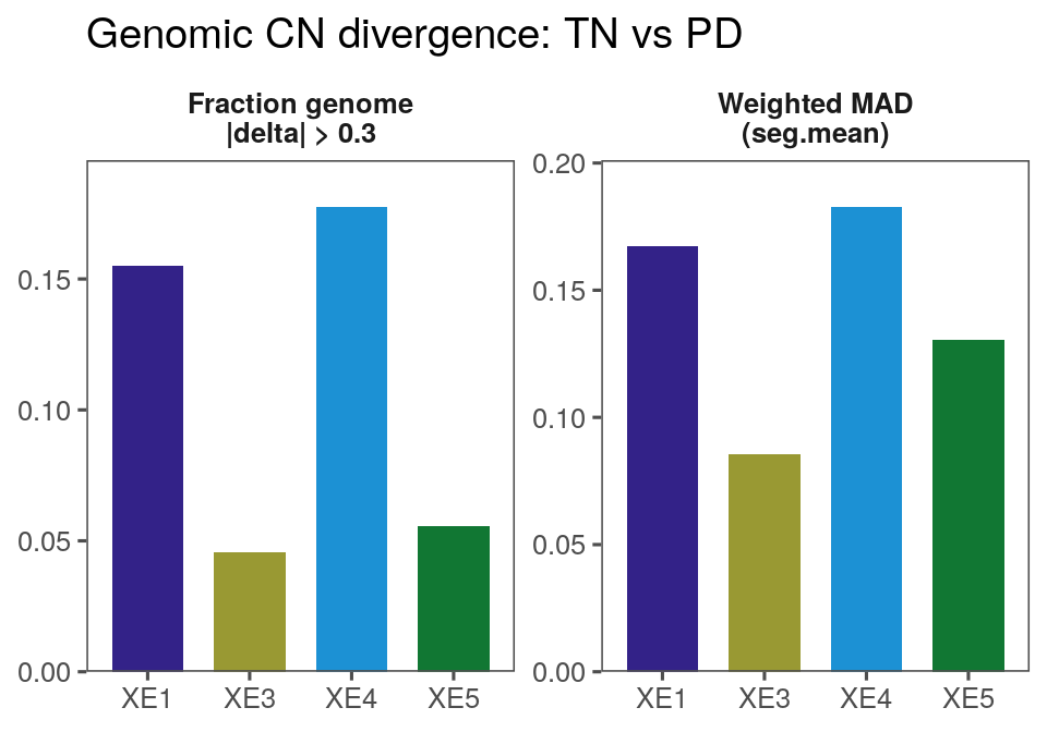
```{r cn-divergence-bar, fig.width = 5, fig.height = 3.5}
p_cn_diff <- cn_diff_results %>%
  dplyr::select(patient_id, wMAD, frac_changed_0.3) %>%
  pivot_longer(-patient_id, names_to = "metric", values_to = "value") %>%
  mutate(
    metric = dplyr::recode(metric,
      "wMAD" = "Weighted MAD\n(seg.mean)",
      "frac_changed_0.3" = "Fraction genome\n|delta| > 0.3"
    ),
    patient_id = factor(patient_id, levels = patients)
  ) %>%
  ggplot(aes(x = patient_id, y = value, fill = patient_id)) +
  geom_col(width = 0.7, show.legend = FALSE) +
  facet_wrap(~metric, scales = "free_y") +
  scale_fill_manual(values = colors$xe_pts, drop = FALSE) +
  # XE2 has no TN/PD pair, so it has no row here; drop = FALSE drew it as an empty bar.
  scale_x_discrete(drop = TRUE) +
  scale_y_continuous(expand = expansion(mult = c(0, 0.1))) +
  labs(x = NULL, y = NULL, title = "Genomic CN divergence: TN vs PD") +
  theme_few() +
  theme(
    strip.background = element_blank(),
    strip.text = element_text(face = "bold")
  )

ggsave(p_cn_diff,
  filename = here("plots", "xenium", "cn_divergence_barplot.pdf"),
  width = 5, height = 3.5
)
p_cn_diff
```
## Fig S12A — cell-type marker dotplot
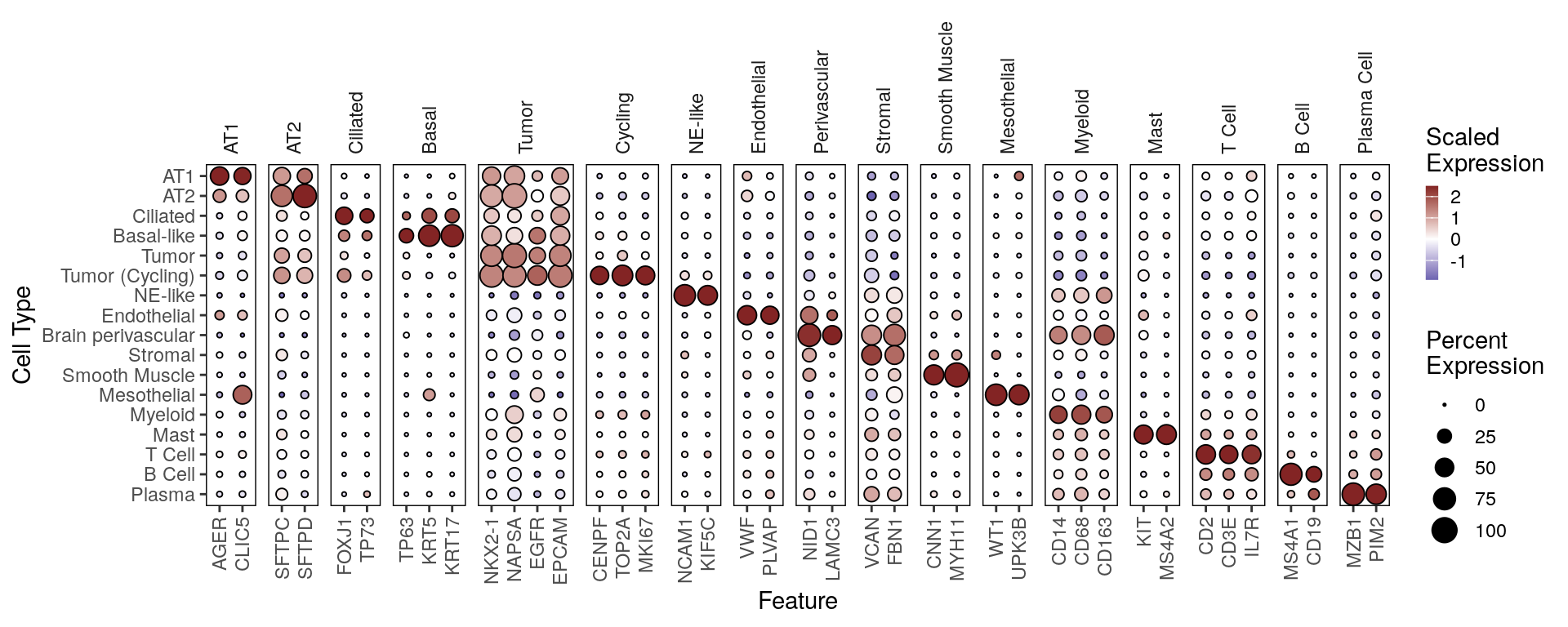
```{r, fig.width = 10, fig.height = 4}
p <- DotPlotter(srt, features = markers$xe_coarse_markers, group.by = "cell_type_detailed", cluster_feats = F, cluster_groups = F, rotate_y_strip = T)
ggsave(p, filename = here("plots", "xenium", "dotplot_coarse_markers.pdf"), width = 10, height = 4)
p
```
## Fig S12B — EGFR mutant-probe positivity barplot
```{r, fig.width = 12, fig.height = 6}
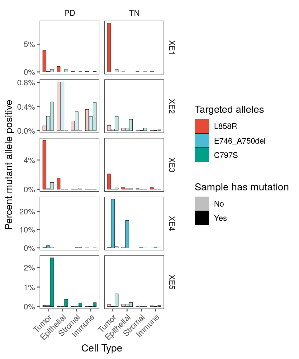
srt$EGFR_L858R_pos <- srt$MUT_L858R > 0
srt$EGFR_E746_A750del_pos <- srt$MUT_E746_A750del > 0
srt$EGFR_C797S_pos <- srt$MUT_C797S_GC > 0

mut_count_df <- srt@meta.data %>%
  group_by(patient_id, sample_id, timepoint) %>%
  mutate(sample_total = n()) %>%
  group_by(cell_type_very_coarse, patient_id, sample_id, timepoint, EGFR.mut, sample_total) %>%
  summarize(
    ct_total = n(),
    EGFR_L858R_pos = sum(EGFR_L858R_pos),
    EGFR_L858R_prop = sum(EGFR_L858R_pos) / n(),
    EGFR_E746_A750del_pos = sum(EGFR_E746_A750del_pos),
    EGFR_E746_A750del_prop = sum(EGFR_E746_A750del_pos) / n(),
    EGFR_C797S_pos = sum(EGFR_C797S_pos),
    EGFR_C797S_prop = sum(EGFR_C797S_pos) / n(),
    .groups = "drop"
  ) %>%
  pivot_longer(
    cols = c(EGFR_L858R_prop, EGFR_E746_A750del_prop, EGFR_C797S_prop),
    names_to = "mutation",
    values_to = "prop"
  ) %>%
  mutate(
    mutation = recode(mutation,
      "EGFR_L858R_prop" = "L858R",
      "EGFR_E746_A750del_prop" = "E746_A750del",
      "EGFR_C797S_prop" = "C797S"
    ),
    is_patient_mutation = case_when(
      mutation == "L858R" & grepl("L858R", EGFR.mut) ~ TRUE,
      mutation == "E746_A750del" & grepl("E746_A750del", EGFR.mut) ~ TRUE,
      mutation == "C797S" & grepl("C797S", EGFR.mut) ~ TRUE,
      .default = FALSE
    )
  )

mut_count_df$mutation <- fct_relevel(mut_count_df$mutation, "L858R", "E746_A750del", "C797S")
```
```{r, fig.width = 5, fig.height = 6}
ct_ord_pt <- c("Tumor", "Epithelial", "Stromal", "Immune")

p <- mut_count_df %>%
  mutate(cell_type_very_coarse = factor(cell_type_very_coarse, levels = ct_ord_pt)) %>%
  ggplot(aes(x = cell_type_very_coarse, y = prop, fill = mutation, alpha = is_patient_mutation)) +
  geom_col(position = position_dodge(width = 0.8), width = 0.7, color = "black", linewidth = 0.15) +
  scale_alpha_manual(
    values = c("TRUE" = 1, "FALSE" = 0.25),
    labels = c("TRUE" = "Yes", "FALSE" = "No"),
    name = "Sample has mutation", drop = F
  ) +
  scale_fill_manual(
    values = c("L858R" = "#E64B35", "E746_A750del" = "#4DBBD5", "C797S" = "#00A087"),
    name = "Targeted alleles"
  ) +
  facet_grid(patient_id ~ timepoint, scales = "free", space = "free_x") +
  theme_few() +
  theme(
    axis.text.x = element_text(angle = 45, hjust = 1),
    strip.background = element_rect(fill = NA, color = "black")
  ) +
  scale_y_continuous(breaks = scales::breaks_extended(n = 3), labels = scales::label_percent()) +
  labs(
    x = "Cell Type",
    y = "Prop. mut+ cells"
  ) +
  guides(alpha = guide_legend(override.aes = list(fill = "black"))) +
  labs(y = "Percent mutant allele positive") +
  theme(legend.position = "right", strip.background = element_blank())
ggsave(p, filename = here("plots", "xenium", "mutation_proportions_by_celltype_patient_grouped.pdf"), width = 5, height = 6)
p
```
## Fig S12C — patient-specificity violin
```{r, fig.width = 4, fig.height = 3}
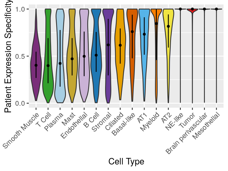
# Read rather than recompute: calc_snn_specificity() subsamples at 10% with no seed, so
# a recompute would not reproduce the published values.
pt_sp <- as.data.frame(data.table::fread(pt_sp_file))

p1 <- pt_sp %>%
  ggplot(aes(x = fct_reorder(cid2, cid1_purity, mean), y = cid1_purity)) +
  geom_violin(scale = "width", aes(fill = cid2), show.legend = F) +
  scale_fill_manual(values = colors$xe_ct) +
  scale_y_continuous(breaks = seq(0, 1, by = 0.5)) +
  geom_pointrange(
    stat = "summary", fatten = 0.8,
    fun.min = function(z) {
      quantile(z, 0.25)
    },
    fun.max = function(z) {
      quantile(z, 0.75)
    },
    fun = median
  ) +
  guides(
    x = guide_axis(angle = 45, cap = "both"),
    y = guide_axis(cap = "both")
  ) +
  labs(x = "Cell Type", y = "Patient Expression Specificity")
ggsave(p1, filename = here("plots", "xenium", "patient_specificity_by_cell_type.pdf"), width = 4, height = 3.2)
p1
```
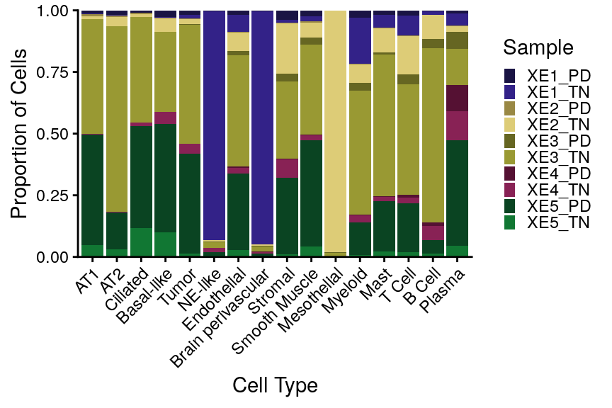
## Fig S12D — cell-type composition
```{r, fig.width = 4.5, fig.height = 3}
p <- srt@meta.data %>%
  ggplot(aes(x = cell_type_coarse, fill = sample_id)) +
  geom_bar(position = "fill") +
  scale_fill_manual(values = colors$xe_tps) +
  labs(x = "Cell Type", y = "Proportion of Cells", fill = "Sample") +
  theme_classic() +
  guides(fill = guide_legend(keywidth = 0.5, keyheight = 0.5)) +
  scale_y_continuous(expand = c(0,0)) +
  theme(axis.text.x = element_text(angle = 45, hjust = 1))
ggsave(p, filename = here("plots", "xenium", "cell_type_composition_by_sample.pdf"), width = 4.5, height = 3)
p
```
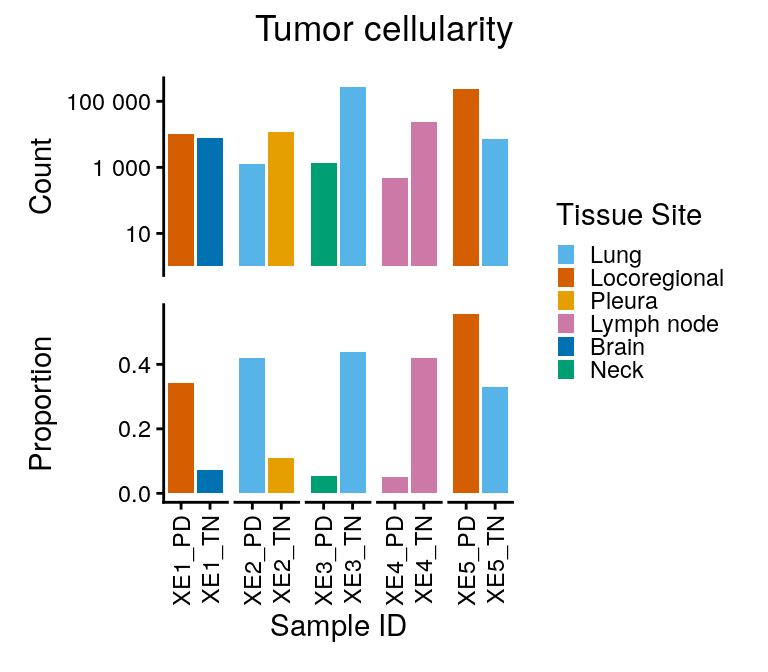
## Fig S12E — tumor count + proportion
```{r, fig.width = 4, fig.height = 3.5}
p1 <- srt@meta.data %>%
  filter(cell_type_coarse == "Tumor") %>%
  ggplot(aes(x = sample_id)) +
  geom_bar(aes(fill = site_of_tissue_simple)) +
  guides(x = guide_axis(angle = 90)) +
  scale_y_log10(breaks = scales::breaks_log(), labels = scales::label_number()) +
  theme_classic() +
  labs(x = "Sample ID", y = "Count")

p2 <- srt@meta.data %>%
  group_by(sample_id, site_of_tissue_simple, patient_id) %>%
  summarize(prop_tumor = mean(cell_type_coarse == "Tumor")) %>%
  ggplot(aes(x = sample_id, y = prop_tumor)) +
  geom_col(aes(fill = site_of_tissue_simple)) +
  guides(x = guide_axis(angle = 90)) +
  scale_y_continuous() +
  theme_classic() +
  labs(x = "Sample ID", y = "Proportion")

pcomb <- p1 + p2 + plot_layout(guides = "collect", axes = "collect", ncol = 1) + plot_annotation(title = "Tumor cellularity", theme = theme(plot.title = element_text(hjust = 0.5), plot.title.position = "panel")) &
  scale_fill_manual(values = colors$site_of_tissue_simple, breaks = names(colors$site_of_tissue_simple)) &
  guides(fill = guide_legend(title = "Tissue Site", keywidth = 0.5, keyheight = 0.5)) &
  facet_grid(.~patient_id, scales = "free", space = "free") &
  theme(strip.text = element_blank(), strip.background = element_blank(),
        panel.spacing = unit(1, "mm"))
ggsave(pcomb, filename = here("plots", "xenium", "tumor_cell_counts_and_proportions_by_sample.pdf"), width = 4, height = 3.5)
pcomb
```
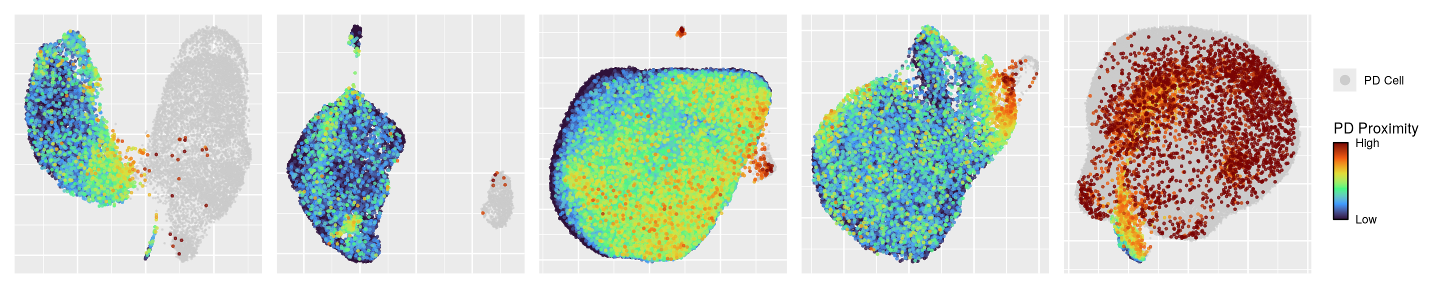
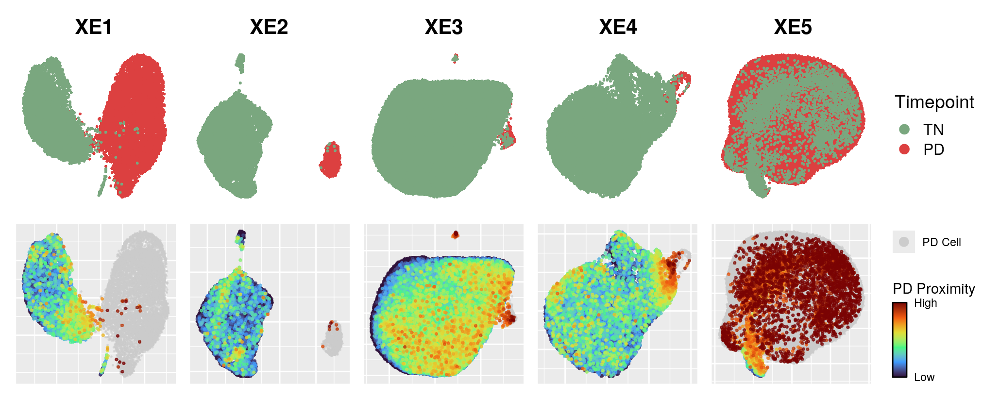
## Fig S13A — timepoint + PD-proximity UMAPs
```{r knn-pd-umap, fig.width = 15, fig.height = 3}
pls_knn <- map(patients, .f = function(pat) {
  xe_tumor <- srt_pts[[pat]]

  umap_embed <- Embeddings(xe_tumor, "umap")
  plot_df <- tibble(
    UMAP_1 = umap_embed[, 1],
    UMAP_2 = umap_embed[, 2],
    timepoint = as.character(xe_tumor$timepoint),
    pd_proximity = xe_tumor$pd_proximity
  )

  df_pd <- plot_df %>% filter(timepoint == "PD")
  df_tn <- plot_df %>% filter(timepoint == "TN") %>% arrange(pd_proximity)

  ggplot() +
    ggrastr::geom_point_rast(data = df_pd, aes(x = UMAP_1, y = UMAP_2, color = timepoint),
               size = 0.1, alpha = 0.5, raster.dpi = 600) +
    scale_color_manual(values = c("PD" = "grey80"),
                       name = NULL,
                       limits = c("PD"),
                       labels = c("PD Cell"),
                       guide = guide_legend(
                         override.aes = list(size = 3, alpha = 1),
                         order = 1
                       )) +
    ggnewscale::new_scale_color() +
    ggrastr::geom_point_rast(data = df_tn, aes(x = UMAP_1, y = UMAP_2, color = pd_proximity),
               size = 0.5, alpha = 0.7, raster.dpi = 600) +
    scale_color_viridis_c(option = "turbo", direction = 1,
                          limits = c(0.3, 0.55),
                          breaks = c(0.3, 0.55),
                          labels = c("Low", "High"),
                          oob = scales::squish,
                          name = "PD Proximity") +
    # `order` pins the collected legend to the published stacking (PD Cell above the
    # PD Proximity colourbar). Without it patchwork is free to swap the two guides.
    guides(color = guide_colorbar(keywidth = 0.75, keyheight = 4,
                                  ticks.colour = "black",
                                  frame.colour = "black",
                                  order = 2)) +
    theme(plot.title = element_text(hjust = 0.5),
          panel.border = element_blank(),
          axis.title = element_blank(),
          axis.ticks = element_blank(),
          axis.text = element_blank(),
          axis.line = element_blank()) +
    NoAxes()
})

wrap_plots(pls_knn, nrow = 1, guides = "collect")
```
```{r}
pls2 <- map(names(srt_pts), .f = function(pat) {
  xe_tumor <- srt_pts[[pat]]
  xe_tumor$timepoint <- factor(xe_tumor$timepoint, levels = c("TN", "PD"))
  p1 <- DimPlot(xe_tumor, reduction = "umap", group.by = c("timepoint"), label = F, order = "TN",
                raster = F) +
    scale_color_manual(name = "Timepoint", values = colors$time_point, breaks = c("TN", "PD")) +
    labs(title = paste(pat),
         x = "UMAP1", y = "UMAP2") +
    NoAxes()
  ggrastr::rasterise(p1, dpi = 1000)
})
names(pls2) <- names(srt_pts)
```
```{r, fig.width = 15/1.4, fig.height = 6/1.4}
pcomb1 <- wrap_plots(pls2, nrow = 1, guides = "collect") & theme(aspect.ratio = 1)
pcomb2 <- wrap_plots(pls_knn, nrow = 1, guides = "collect") & theme(aspect.ratio = 1)

pcomb <- pcomb1 / pcomb2
ggsave(pcomb, filename = here("plots", "xenium", "pd_like_tn_umaps.pdf"), width = 15/1.4, height = 6/1.4)
pcomb
```
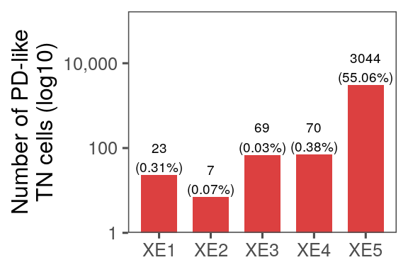
## Fig S13B — PD-like TN count barplot
```{r, fig.width = 10, fig.height = 3}
fts <- rownames(srt_epi)
df_preres <- FetchData(srt_epi[, srt_epi$cell_type_coarse == "Tumor"],
                        vars = c("cell_id", "patient_id", "nCount_RNA",
                                 "mut_pos_cell", "timepoint", "cell_type_coarse",
                                 fts, grep("_score$", colnames(srt_epi@meta.data), value = TRUE)))
df_preres$timepoint <- fct_relevel(df_preres$timepoint, "TN", "PD")

df_preres <- left_join(df_preres, knn_results)

df_preres$category <- case_when(
  df_preres$timepoint == "PD" ~ "PD",
  df_preres$pd_like_tn ~ "TN (PD-like)",
  df_preres$timepoint == "TN" ~ "TN",
  TRUE ~ "Other"
)

df_preres$category <- fct_relevel(df_preres$category, "TN", "TN (PD-like)", "PD")
```
```{r, fig.width = 3, fig.height = 2}
bar_df <- df_preres %>%
  filter(timepoint == "TN") %>%
  mutate(pd_like_label = if_else(pd_like_tn, "PD-like TN", "TN-like TN")) %>%
  count(patient_id, pd_like_label) %>%
  group_by(patient_id) %>%
  mutate(
    total = sum(n),
    prop  = n / total
  ) %>%
  ungroup()

p <- ggplot(bar_df %>% filter(pd_like_label == "PD-like TN"),
       aes(x = patient_id, y = n, fill = pd_like_label)) +
  geom_col(width = 0.7) +
  geom_text(aes(label = glue::glue("{n}\n({scales::percent(prop, accuracy = 0.01)})")),
            vjust = -0.1, size = 2.5) +
  scale_fill_manual(values = c("PD-like TN" = colors$time_point[["PD"]])) +
  scale_y_log10(labels = scales::comma, expand = expansion(mult = c(0, 0.5))) +
  labs(x = NULL, y = "Number of PD-like\nTN cells (log10)", fill = NULL) +
  theme_few() +
  theme(legend.position = "none")
ggsave(p, filename = here("plots", "xenium", "pd_like_tn_barplot_counts.pdf"), width = 3, height = 2)
p
```
## Fig S13C — lineage-score line plots
```{r}
sel_mrks <- c("alveolar_score", "basal_squamous_score", "neuroendocrine_score",
          "NKX2-1", "SFTPB", "SFTPC", "NAPSA", "CLIC5",
          "SOX2", "SOX4", "SOX9", "TP63", "KRT5", "KRT14",
          "DUSP6",
          lung_lineage_genes$alveolar, lung_lineage_genes$basal_squamous,
          lung_lineage_genes$neuroendocrine
          ) %>%
  unique()

df_preres_med <- df_preres %>%
  pivot_longer(cols = any_of(sel_mrks), names_to = "feature", values_to = "value") %>%
  group_by(patient_id, category, feature) %>%
  summarize(median_val = median(value, na.rm = TRUE), .groups = "drop") %>%
  mutate(category = fct_relevel(category, "TN", "TN (PD-like)", "PD"))

pls_med_lines <- setNames(
  lapply(sel_mrks, function(ft) {
    df_preres_med %>%
      filter(feature == ft) %>%
      ggplot(aes(x = category, y = median_val, group = patient_id)) +
      geom_line(aes(color = patient_id), linewidth = 0.5) +
      geom_point(aes(fill = patient_id), size = 2.5, pch = 21) +
      scale_fill_manual(values  = colors$xe_pts) +
      scale_color_manual(values = colors$xe_pts) +
      scale_x_discrete(expand = c(0.1, 0.1)) +
      theme_few() +
      guides(fill = guide_legend(ncol = 1),
             x = guide_axis(angle = 45)) +
      labs(fill = "Patient", color = "Patient",
           y = ft, x = NULL) +
      theme(panel.grid.minor = element_blank(),
            legend.position = "right",
            strip.clip = "off")
  }),
  sel_mrks
)
```
```{r}
# Right panel: median per-cell PD-axis position (no bootstrap needed — full data)
p_axis_lines <- percell_sims %>%
  mutate(category = fct_relevel(category, "TN", "TN (PD-like)", "PD")) %>%
  group_by(patient_id, category) %>%
  summarize(median_pd_axis = median(pd_axis), .groups = "drop") %>%
  ggplot(aes(x = category, y = median_pd_axis, group = patient_id)) +
  geom_line(aes(color = patient_id), linewidth = 0.7) +
  geom_point(aes(fill = patient_id), size = 3, pch = 21) +
  scale_fill_manual(values = colors$xe_pts) +
  scale_color_manual(values = colors$xe_pts) +
  labs(x = NULL, y = "Transcriptional similarity to PD",
       title = "TN(PD-like) is transcriptionally intermediate",
       fill = "Patient", color = "Patient") +
  theme_few()
```
```{r, fig.width = 4, fig.height = 2.5}
p_axis_lines2 <- p_axis_lines +
  scale_x_discrete(expand = c(0.1, 0.1)) +
  labs(title = NULL)
p_axis_lines2
```
```{r, fig.width = 10, fig.height = 2.5}
pcomb <-
  (p_axis_lines2 + labs(y = "Median PD similarity") + theme(legend.position = "none") + guides(x = guide_axis(angle = 45))) +
  (pls_med_lines$alveolar_score + labs(y = "Alveolar score")) +
  (pls_med_lines$basal_squamous_score + labs(y = "Basal squamous score")) +
  (pls_med_lines$neuroendocrine_score + labs(y = "Neuroendocrine score")) +
  plot_layout(nrow = 1, guides = "collect")
ggsave(pcomb, file = here("plots", "xenium", "preres_median_lineplots2.pdf"), width = 10, height = 2.5)
pcomb
```
## Fig S13D — spatial PD-like localization
```{r}
colors$pdlike_cols <- c(
  Tumor = "#e31a1c",
  `PD-like Tumor` = "#FF8C00",
  AT1 = "#56B4E9",
  AT2 = "#F0E442",
  Ciliated = "#E69F00",
  `Basal-like` = "#D55E00",
  `NE-like` = "#1C91D4",
  Endothelial = "#cab2d6",
  `Brain perivascular` = "#B39DDB",
  Stromal = "#6a3d9a",
  `Smooth Muscle` = "#7A2E7A",
  Mesothelial = "#999999",
  Myeloid = "#ff7f00",
  Mast = "#c4a731",
  `T Cell` = "#33a02c",
  `B Cell` = "#1f78b4",
  Plasma = "#a6cee3",
  "Other" = "grey50"
)
```
```{r}
xe1_tn_select <- read.csv(xe1_region_file, header = T, skip = 2)

# cell_type_pdlike / cell_type_pdlike_simple are baked into the object

ft_list <- c(
  "EGFR", "NKX2-1", "SFTPB", "HOPX", "NAPSA", # Alveolar/LUAD
  "DUSP6", "MET", "FGFR3", "ERBB2",
  "ASCL1", "CHGA", "NCAM1", "SYP", # NE
  "XPO1", "alveolar_score", "basal_squamous_score", "neuroendocrine_score"
)
feat_df <- FetchData(srt, vars = c("cell_id", ft_list))

df <- map(unique(srt$sample_id), .f = function(fov) {
  GetTissueCoordinates(srt, image = fov)
}) %>%
  list_rbind() %>%
  dplyr::rename(cell_id = cell) %>%
  inner_join(srt@meta.data) %>%
  filter(!is.na(cell_type_coarse)) %>%
  left_join(feat_df)

df <- split(df, df$sample_id)

df$XE1_TN <- df$XE1_TN %>%
  filter(barcode %in% xe1_tn_select$Cell.ID)
```
```{r, fig.width = 16, fig.height = 4}
# Scale bar length in mm per sample (coordinates are in μm, 1 mm = 1000 μm)
scale_bar_mm <- c(
  "XE1_TN" = 1,
  "XE2_TN" = 1,
  "XE3_TN" = 1,
  "XE4_TN" = 1,
  "XE5_TN" = 1
)

add_scale_bar_mm <- function(p, spec, bar_mm) {
  bar_um <- bar_mm * 1000
  xr   <- spec$x
  yr   <- spec$y
  xpad <- diff(xr) * 0.02
  ypad <- diff(yr) * 0.02
  x0   <- xr[1] + xpad
  x1   <- x0 + bar_um
  ybar <- yr[1] + ypad
  ylab <- ybar + diff(yr) * 0.06

  box_xpad <- diff(xr) * 0.02
  box_ypad <- diff(yr) * 0.02
  box_x0   <- x0 - box_xpad
  box_x1   <- x1 + box_xpad
  box_y0   <- ybar - box_ypad
  box_y1   <- ylab + diff(yr) * 0.03

  p +
    annotate("rect", xmin = box_x0, xmax = box_x1, ymin = box_y0, ymax = box_y1,
             fill = "white", color = NA, alpha = 0.8) +
    annotate("segment", x = x0, xend = x1, y = ybar, yend = ybar,
             color = "black", linewidth = 1.4) +
    annotate("text", x = (x0 + x1) / 2, y = ylab,
             label = paste0(bar_mm, "mm"),
             color = "black", size = 3, hjust = 0.5)
}

# Draw each layer separately to avoid overplotting
pls_pdlike <- map(grep("TN", names(df), value = T), .f = function(samp) {
  fov_spec <- list(
    x = range(df[[samp]]$x, na.rm = TRUE),
    y = range(df[[samp]]$y, na.rm = TRUE)
  )

  p <- df[[samp]] %>%
    ggplot(aes(x = x, y = y)) +
    scattermore::geom_scattermore(
      data = df[[samp]][df[[samp]]$cell_type_pdlike_simple == "Other",],
      aes(color = cell_type_pdlike_simple), pointsize = 1, alpha = 0.5
      ) +
    scattermore::geom_scattermore(
      data = df[[samp]][df[[samp]]$cell_type_pdlike_simple == "Tumor",],
      aes(color = cell_type_pdlike_simple), pointsize = 1.5, alpha = 1
      ) +
    geom_point(data = df[[samp]][df[[samp]]$cell_type_pdlike_simple == "PD-like Tumor",],
               aes(fill = cell_type_pdlike_simple), size = 1.5, pch = 21, alpha = 1) +
    scale_color_manual(values = colors$pdlike_cols) +
    scale_fill_manual(values = colors$pdlike_cols) +
    labs(title = samp,
         fill = "Cell Type", color = "Cell Type") +
    theme_void() +
    theme(panel.border = element_rect(fill = NA, color = "black", linewidth = 1),
          plot.title = element_text(hjust = 0.5, face = "bold", size = 16),
          plot.margin = margin(5.5,5.5,5.5,5.5))

  p <- add_scale_bar_mm(p, fov_spec, bar_mm = scale_bar_mm[[samp]])
  p
})

pcomb <- wrap_plots(pls_pdlike, nrow = 1, guides = "collect") &
  theme(aspect.ratio = 1)
ggsave(pcomb, file = here("plots", "xenium", "pd_like_tn_spatial.pdf"), width = 16, height = 4)
pcomb
```
## Session info
```{r session-info}
sessionInfo()
```