---
title: "Figure 4 and S9 -- adenocarcinoma cell identity is coupled to MAPK signaling"
author: "Matthew Zatzman"
execute:
warning: false
error: false
format:
html:
code-fold: true
code-tools: true
toc: true
---
Figure 4 and Supplementary Figure S9 (lineage signatures and MAPK pathway
activity).
S9B reuses the correlation table built for Figure 4B, so those chunks stay
together in this document.
Run `00_download_convert.qmd` first to build `paper_data/`.
{{< include _setup.qmd >}}
# Load data
The epithelial and tumor objects.
```{r load}
# L'Ecuyer-CMRG so forked mclapply workers get reproducible streams.
RNGkind("L'Ecuyer-CMRG")
set.seed(42)

db <- load_project(objects = c("epi", "tum"))

srt_epi <- db$srt_epi
srt_tum <- db$srt_tum
```
## Cohort metadata, pathways and IHC
`metadata` is Table S1 as published: one row per reported specimen, 73 rows. The
two-core MRD2 merge is already applied both here and in the objects, so nothing in
this notebook needs to reconcile libraries against specimens.
```{r metadata}
metadata <- readxl::read_excel(here("paper_data", "supplemental_tables.xlsx"),
                               sheet = "Table S1 - Cohort Metadata") %>%
  as.data.frame()
for (v in c("facets_fga", "facets_ploidy", "facets_purity", "facets_frac_loh")) {
  metadata[[v]] <- as.numeric(metadata[[v]])
}
metadata$facets_wgd <- as.logical(metadata$facets_wgd)
metadata$time_point <- fct_relevel(metadata$time_point, "TN", "MRD", "PD")
metadata$sample_id  <- fct_relevel(metadata$sample_id, names(colors$sample_id))
stopifnot(nrow(metadata) == 73, !any(duplicated(metadata$sample_id)))

# Sample-level view used by the composition and cellularity panels.
meta_final <- metadata
meta_final$sample_has_tumor <- meta_final$sample_id %in% unique(srt_tum$sample_id)
```
```{r pathways}
pathways <- read.table(here("paper_data", "egfr_pathways_annotations.txt"),
                       header = TRUE, sep = "\t")
mapk_paths <- filter(pathways, category == "MAPK")$pathway
tum_paths  <- c("LUAD", "LUSC", "SCLC")

# The signature columns on the objects use the short names; the pathway tables use the
# source names. Rename the tables, not the objects.
rename_sigs <- function(df) {
  df$pathway[df$pathway == "LUAD_GIRARD"] <- "LUAD"
  df$pathway[df$pathway == "LUSC_GIRARD"] <- "LUSC"
  df$pathway[df$pathway == "SCLC_CCLE"]   <- "SCLC"
  df
}
pathways <- rename_sigs(pathways)

# Named separately because S9A/S9E use its gene lists directly. Deliberately not passed
# through rename_sigs() -- the v2 names are what the GSEA TERM2GENE mapping expects.
pathways_v2 <- read.table(here("paper_data", "egfr_pathways_v2.txt"),
                          header = TRUE, sep = "\t")
pathways_v2_t2g <- pathways_v2 %>% dplyr::relocate(pathway, Gene)

# pathways_full adds the v2 set and the 67 Tirosh metaprograms, which together define the
# `mp*` score columns carried on srt_epi / srt_tum.
pathways_full <- bind_rows(
  pathways_v2,
  read.csv(here("paper_data", "tirosh_mps_67_natcan_2025.csv")) %>%
    dplyr::rename(pathway = Geneset) %>%
    dplyr::select(pathway, Gene)
) %>% rename_sigs()
```
The IHC table is keyed on `sample_id`, so it joins to `meta_final` directly. It covers 24
of the 73 specimens; the rest were not stained.
```{r ihc}
ihc <- readr::read_csv(here("paper_data", "nucseq_ihc_public.csv"),
                       show_col_types = FALSE) %>%
  # The source column is misspelled "cytoplsmic". Without this rename it fails
  # ends_with("_cytoplasmic") below and is silently left out of the pivot, and since the
  # S7B panel then drops DUSP6 Nuclear as well, DUSP6 disappears from `gene` entirely and
  # fct_relevel(gene, sel_stains) errors on the absent level. Upstream renames it too.
  dplyr::rename("dusp6_cytoplasmic" = "dusp6_cytoplsmic") %>%
  inner_join(meta_final, by = "sample_id") %>%
  dplyr::relocate(sample_id, time_point, scrna_histology, .before = 1)

ihc_long <- ihc %>%
  pivot_longer(cols = c(ends_with("_cytoplasmic"), ends_with("_nuclear")),
               values_to = "value", names_to = "stain") %>%
  mutate(value = as.numeric(value)) %>%
  mutate(
    gene = str_to_upper(gsub("_cytoplasmic|_nuclear", "", stain)),
    stain_loc = ifelse(grepl("cytoplasmic", stain), "Cytoplasmic", "Nuclear"),
    time_point = fct_relevel(time_point, "TN", "MRD")
  ) %>%
  filter(!is.na(value), !is.na(time_point)) %>%
  group_by(stain) %>%
  mutate(value_z = scale(value)[, 1]) %>%
  ungroup() %>%
  mutate(gene_lab = ifelse(stain_loc == "Cytoplasmic", glue("{gene} (C)"), glue("{gene} (N)"))) %>%
  mutate(osi_exp = ifelse(time_point %in% c("MRD", "PD"), "Exp", "TN")) %>%
  filter(sample_id %in% srt_tum$sample_id) %>%
  mutate(score_cat = case_when(
    value < 10 ~ "Negative",
    value >= 10 & value < 100 ~ "Low",
    value >= 100 & value < 200 ~ "Medium",
    value >= 200 ~ "High"
  )) %>%
  mutate(score_cat = factor(score_cat, levels = c("Negative", "Low", "Medium", "High")))

meta_final$has_ihc <- meta_final$sample_id %in% ihc_long$sample_id
```
# Figure 4 -- Adenocarcinoma cell identity is coupled to MAPK signaling
## Figure 4A -- MAPK vs LUAD signature across specimens
Reconstruct `all_sig_summary` from `srt_epi` so this section is self-contained
(does not require the upstream signature heatmap chunks to have been run).
```{r mapk_rebuild_all_sig_summary}
# --- Define pathway groups from srt_epi metadata columns ---
emt_paths <- grep("emt|HALLMARK_EPITHELIAL_MESENCHYMAL_TRANSITION", colnames(srt_epi@meta.data), ignore.case = T, value = T)
myc_paths <- grep("myc", colnames(srt_epi@meta.data), ignore.case = T, value = T)
stemness <- c("WONG_EMBRYONIC_STEM_CELL_CORE", "BENPORATH_PRC2_TARGETS")
metabolic_paths <- c("HALLMARK_GLYCOLYSIS", "HALLMARK_OXIDATIVE_PHOSPHORYLATION", "HALLMARK_MTORC1_SIGNALING")
histological_malignant <- c("LUAD", "LUSC", "SCLC")
histological <- c("TRAVAGLINI_LUNG_ALVEOLAR_EPITHELIAL_TYPE_1_CELL", "TRAVAGLINI_LUNG_ALVEOLAR_EPITHELIAL_TYPE_2_CELL", "mp44_alveolar", "TRAVAGLINI_LUNG_BASAL_CELL", "TRAVAGLINI_LUNG_CILIATED_CELL", "TRAVAGLINI_LUNG_CLUB_CELL", "TRAVAGLINI_LUNG_NEUROENDOCRINE_CELL", "TRAVAGLINI_LUNG_PROLIFERATING_BASAL_CELL", "TRAVAGLINI_LUNG_PROXIMAL_BASAL_CELL", "TRAVAGLINI_LUNG_GOBLET_CELL", "TRAVAGLINI_LUNG_MUCOUS_CELL", "TRAVAGLINI_LUNG_MESOTHELIAL_CELL")
cell_cycle <- grep("cycle", colnames(srt_epi@meta.data), ignore.case = T, value = T)
mapk <- c("REACTOME_MAPK_FAMILY_SIGNALING_CASCADES", "REACTOME_MAPK_TARGETS_NUCLEAR_EVENTS_MEDIATED_BY_MAP_KINASES", "BIOCARTA_MAPK_PATHWAY", "KEGG_MAPK_SIGNALING_PATHWAY", "REACTOME_SIGNALING_BY_EGFR")

pth_list <- list(
  "EMT" = emt_paths,
  "MYC" = myc_paths,
  "Stem" = stemness,
  "Metabolic" = metabolic_paths,
  "Lung Cancer" = histological_malignant,
  "Histological" = histological,
  "Cell Cycle" = cell_cycle,
  "MAPK" = mapk
)

# --- Resolve to features actually present in srt_epi metadata ---
all_meta_cols <- colnames(srt_epi@meta.data)
select_paths <- unique(unlist(pth_list))
select_paths <- select_paths[select_paths %in% all_meta_cols]

# Apply same exclusions as the heatmap pipeline
select_paths <- select_paths[!grepl("_epithelial$", select_paths)]
select_paths <- select_paths[!grepl("TGFB", select_paths)]
# Remove extra curated MYC pathways (keep only mp27_myc and Hallmark)
curated_myc <- select_paths[grepl("MYC", select_paths, ignore.case = TRUE) &
                              !grepl("^mp|^HALLMARK_", select_paths)]
select_paths <- setdiff(select_paths, curated_myc)

# --- Build category map (feature → category) ---
pth_category_df <- enframe(pth_list, name = "feature.groups", value = "features.plot") %>%
  unnest(cols = "features.plot") %>%
  filter(features.plot %in% select_paths) %>%
  distinct(features.plot, .keep_all = TRUE)

# Pathway renaming now uses egfrnucseq::rename_pathway() (see R/utils.R) so this
# logic stays consistent across the document instead of being duplicated
# inline in every section.

# --- Build pathway_category_map (pathway name → feature.groups) ---
pathway_category_map <- pth_category_df %>%
  mutate(pathway = rename_pathway(features.plot)) %>%
  distinct(pathway, feature.groups)

# --- Build all_sig_summary ---
all_sig_summary <- srt_epi@meta.data %>%
  filter(is_tumor_cell) %>%
  group_by(sample_id, time_point) %>%
  summarize(across(all_of(select_paths), ~ mean(.x, na.rm = TRUE)), .groups = "drop") %>%
  pivot_longer(cols = all_of(select_paths), names_to = "features.plot", values_to = "Score") %>%
  group_by(features.plot) %>%
  mutate(Score_Scaled = scale(Score)[, 1]) %>%
  ungroup() %>%

  mutate(pathway = rename_pathway(features.plot)) %>%
  left_join(pathway_category_map, by = "pathway")

# --- Define category and pathway ordering (used by stats/plotting) ---
pth_cat_order <- c(
  "Histological", "Lung Cancer", "MAPK", "EMT", "MYC",
  "Stem", "Metabolic", "Cell Cycle"
)

pth_order <- c(
  "G1S", "G2M", "G2M Score", "HMG Rich", "S Score",
  "EMT (I)", "EMT (II)", "EMT (III)", "EMT (IV)", "EMT (V)", "EMT (VI)",
  "LUAD", "LUSC", "SCLC",
  "AT1 Cell", "AT2 Cell", "Alveolar Signature", "Basal Cell", "Proximal Basal Cell",
  "Proliferating Basal Cell", "Goblet Cell", "Mucous Cell", "Club Cell", "Mesothelial Cell", "Ciliated Cell",
  "Neuroendocrine Cell", "MYC", "MYC Targets V1", "MYC Targets V2",
  "Glycolysis", "OxPhos", "MTORC1", "ESC",
  "PRC2 Targets",
  "Nuclear MAPK (Reactome)", "MAPK (KEGG)", "MAPK (Biocarta)", "MAPK (Reactome)", "EGFR (Reactome)"
)

# --- Compute unified statistics ---
all_sig_stats <- all_sig_summary %>%
  group_by(pathway) %>%
  rstatix::wilcox_test(Score ~ time_point) %>%
  ungroup() %>%
  mutate(p.adj = p.adjust(p, method = "BH")) %>%
  rstatix::add_significance("p.adj")

# Add y positions for plotting
comparison_order <- tibble(
  group1 = c("TN", "MRD", "TN"),
  group2 = c("MRD", "PD", "PD"),
  comp_rank = c(1, 3, 2)
)

all_sig_stats <- all_sig_summary %>%
  group_by(pathway) %>%
  summarize(max_score = max(Score, na.rm = TRUE), .groups = "drop") %>%
  right_join(all_sig_stats, by = "pathway") %>%
  left_join(comparison_order, by = c("group1", "group2")) %>%
  group_by(pathway) %>%
  arrange(pathway, comp_rank) %>%
  mutate(y.position = max_score * (1.05 + 0.08 * (comp_rank - 1))) %>%
  ungroup() %>%
  dplyr::select(-comp_rank)

# Also define select_paths_name (the cleaned pathway names) for downstream use
select_paths_name <- unique(all_sig_summary$pathway)

cli::cli_alert_success("Rebuilt all_sig_summary ({nrow(all_sig_summary)} rows, {n_distinct(all_sig_summary$pathway)} pathways) and all_sig_stats ({nrow(all_sig_stats)} tests)")
```
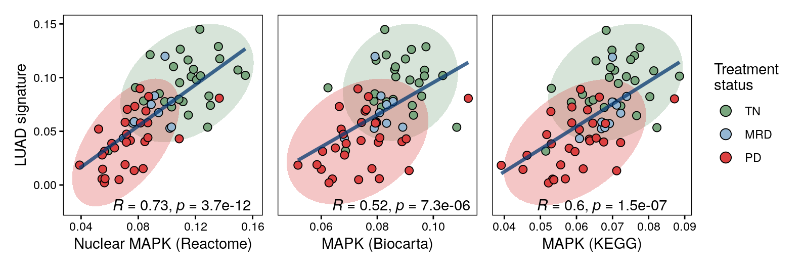
Supervised pathway correlations
```{r fig4a-luad-mapk-select-cors, fig.width = 8.25, fig.height = 2.75}
paths <- c("Nuclear MAPK (Reactome)", "MAPK (Biocarta)", "MAPK (KEGG)")
all_sig_summary_wide <- all_sig_summary %>%
  pivot_wider(id_cols = c("sample_id", "time_point"), names_from = pathway, values_from = Score)

pls <- map(paths, .f = function(pth) {
  p <- all_sig_summary_wide %>%
    ggplot(aes(x = .data[[pth]], y = LUAD)) +
    stat_ellipse(
      data = all_sig_summary_wide[all_sig_summary_wide$time_point != "MRD", ],
      aes(fill = time_point),
      type = "t",
      geom = "polygon",
      alpha = 0.3, show.legend = F
    ) +
    geom_point(aes(fill = time_point), pch = 21, stroke = 0.5, size = 2.5) +
    geom_line(stat = "smooth", method = "lm", color = "#063970", se = F, linewidth = 1.25, alpha = 0.75) +
    ggpubr::stat_cor(label.x.npc = 0.2, label.y = -0.02) +
    scale_fill_manual(values = colors$time_point, breaks = names(colors$time_point)) +
    # scale_color_manual(values = colors$time_point) +
    theme_classic() +
    labs(y = "LUAD signature", fill = "Treatment\nstatus", x = pth) +
    guides(fill = guide_legend(override.aes = list(size = 3.5)))
})

pcomb <- wrap_plots(pls, nrow = 1, guides = "collect", axes = "collect", axis_titles = "collect") & theme(panel.border = element_rect(fill = NA, color = "black"), axis.line = element_blank())
ggsave(pcomb, file = here("plots", "luad_mapk_select_cors.pdf"), width = 8.25, height = 2.75)
pcomb
```
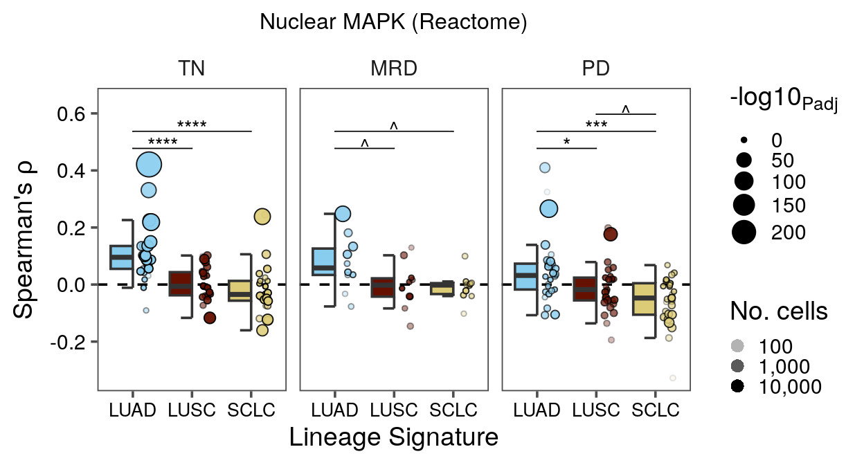
## Figure 4B -- within-specimen nuclear MAPK vs lineage correlations
```{r}
library(easystats)

# Named rather than left in `x`: this table is read by both Figure 4B and Figure S9B,
# which the manuscript ordering separates by the whole of Figure 4. A scratch name would
# be silently clobbered in between.
per_sample_cor <- srt_epi@meta.data %>%
  filter(is_tumor_cell) %>%
  mutate(sample_id = factor(sample_id)) %>%
  add_count(sample_id, name = "n_cells") %>%
  dplyr::group_by(sample_id) %>%
  correlation::correlation(select = c("LUAD", "LUSC", "SCLC"), select2 = c("BIOCARTA_MAPK_PATHWAY", "KEGG_MAPK_SIGNALING_PATHWAY", "REACTOME_MAPK_TARGETS_NUCLEAR_EVENTS_MEDIATED_BY_MAP_KINASES"), method = "spearman") %>%
  left_join(distinct(srt_epi@meta.data[, c("sample_id", "time_point")]), by = c("Group" = "sample_id")) %>%
  mutate(
    mapk_path = case_when(
      Parameter2 == "BIOCARTA_MAPK_PATHWAY" ~ "MAPK (Biocarta)",
      Parameter2 == "KEGG_MAPK_SIGNALING_PATHWAY" ~ "MAPK (KEGG)",
      Parameter2 == "REACTOME_MAPK_TARGETS_NUCLEAR_EVENTS_MEDIATED_BY_MAP_KINASES" ~ "Nuclear MAPK (Reactome)",
      .default = Parameter2
    )
  )
```
```{r fig4b-per-sample-mapk-cor-main, fig.width = 6.5, fig.height = 3.5}
p <- per_sample_cor %>%
  filter(Parameter2 == "REACTOME_MAPK_TARGETS_NUCLEAR_EVENTS_MEDIATED_BY_MAP_KINASES") %>%
  arrange(desc(p)) %>%
  ggplot(aes(x = Parameter1, y = rho)) +
  geom_hline(yintercept = 0, linetype = "dashed") +
  gghalves::geom_half_boxplot(outliers = F, aes(fill = Parameter1), errorbar.draw = T) +
  gghalves::geom_half_point_panel(aes(size = -log10(p), fill = Parameter1, alpha = n_Obs),
                                  transformation = position_jitter(width = 0.5), pch = 21) +
  facet_grid(. ~ time_point) +
  scale_fill_manual(values = colors$histology_predominant_short) +
  scale_alpha_continuous(trans = "log10", breaks = scales::breaks_log(), labels = scales::label_number(big.mark = ",")) +
  guides(
    fill = "none",
    x = guide_axis(angle = 0),
    size = guide_legend(override.aes = list(pch = 19), keywidth = 0, keyheight = 0),
    alpha = guide_legend(override.aes = list(pch = 16, size = 3), keywidth = 0, keyheight = 0)
  ) +
  ggpubr::geom_pwc(tip.length = 0, label = "p.adj.signif", step.increase = 0.08, vjust = 0.5, hide.ns = T, bracket.nudge.y = 0.075, symnum.args = symnum_0.1_star) +
  scale_y_continuous(expand = expansion(mult = c(0.05, 0.1))) +
  theme_few(base_size = 14) +
  theme(
    strip.clip = "off",
    plot.title = element_text(hjust = 0.5, size = 12),
    plot.title.position = "panel",
    axis.text = element_text(color = "black"),
    axis.text.x = element_text(size = 10),
    # strip.text.y.right = element_text(size = 12, angle = 90)
  ) +
  labs(x = "Lineage Signature",
       y = bquote("Spearman's" ~ rho),
       size = bquote("-log10"[Padj]),
       alpha = "No. cells",
       title = "Nuclear MAPK (Reactome)")
ggsave(p, file = here("plots", "per_sample_mapk_cor_main.pdf"), width = 6.5, height = 3.5)
p
```
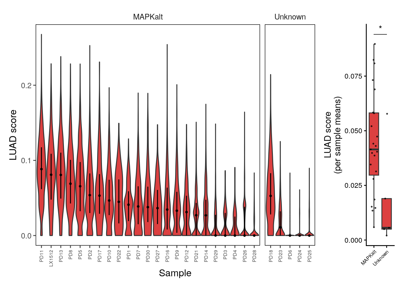
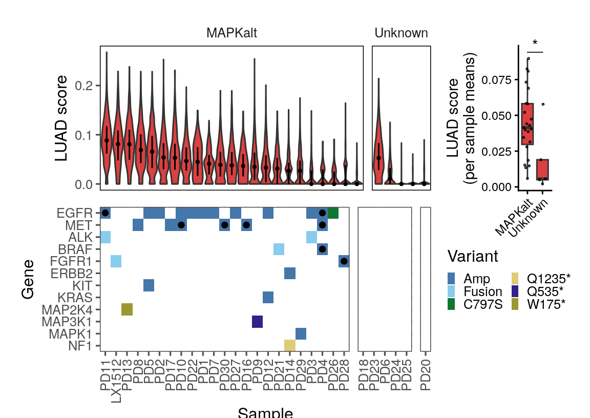
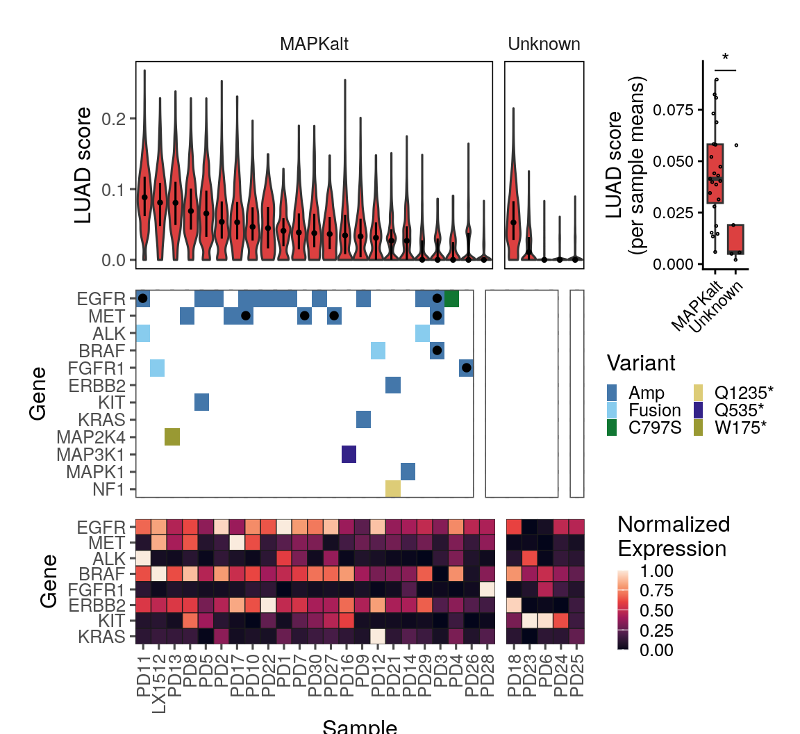
## Figure 4E and 4F -- LUAD score, MAPK oncoprint and expression in PD
LUAD score per PD specimen, split by whether a secondary MAPK alteration was called.
```{r}
samp_ord <- srt_tum@meta.data %>%
  filter(time_point == "PD", !is.na(mapk_alt)) %>%
  mutate(sample_id = fct_reorder(sample_id, -LUAD, median)) %>%
  pull(sample_id) %>%
  levels()

p1 <- srt_tum@meta.data %>%
  filter(time_point == "PD", !is.na(mapk_alt)) %>%
  ggplot(aes(x = fct_relevel(sample_id, samp_ord), y = LUAD)) +
  # ggplot(aes(x = sample_id, y = LUAD)) +

  geom_violin(scale = "width", aes(fill = time_point), show.legend = F) +
  geom_pointrange(
    stat = "summary", fatten = 0.1,
    fun.min = function(z) {
      quantile(z, 0.25)
    },
    fun.max = function(z) {
      quantile(z, 0.75)
    },
    fun = median, position = position_dodge(width = 0.8)
  ) +
  facet_grid(. ~ mapk_alt, scales = "free", space = "free") +
  guides(x = guide_axis(angle = 90)) +
  labs(x = "Sample", y = "LUAD score") +
  scale_fill_manual(values = colors$time_point) +
  theme_few() +
  theme(
    axis.line = element_blank(),
    panel.border = element_rect(fill = NA, color = "black"),
    strip.background.x = element_blank()
  )

p2 <- srt_tum@meta.data %>%
  filter(time_point == "PD", !is.na(mapk_alt)) %>%
  group_by(sample_id, mapk_alt, time_point) %>%
  summarize(LUAD = mean(LUAD)) %>%
  ggplot(aes(x = mapk_alt, y = LUAD)) +
  geom_boxplot(outliers = F, aes(fill = time_point), show.legend = F) +
  geom_quasirandom(size = 0.3, pch = 1) +
  ggpubr::geom_pwc(tip.length = 0, label = "p.signif") +
  guides(x = guide_axis(angle = 45)) +
  scale_fill_manual(values = colors$time_point) +
  labs(x = NULL, y = "LUAD score\n(per sample means)") +
  coord_cartesian(clip = "off") +
  theme_classic()

pcomb <- p1 + p2 + plot_layout(nrow = 1, widths = c(1, 0.1), guides = "collect") & theme(axis.text.x = element_text(size = 6))
pcomb
```
Create a plot with the mutations annotated in a bar on the side, and notable genes expression in a box heat encoding
```{r, fig.width = 6, fig.height = 4.25}
mapk_alt_df <- meta_final[,c("sample_id", "time_point", "secondary_mapk", "mapk_alt")] %>%
  filter(!is.na(mapk_alt), sample_id %in% unique(srt_tum$sample_id)) %>%
  separate_rows(secondary_mapk, sep = ", ") %>%
  separate(secondary_mapk, sep = "_", into = c("Gene", "Variant_Type"), remove = F) %>%
  mutate(
    infercnv = grepl("inf", Variant_Type),
    Variant_Type = gsub("inf", "", Variant_Type),
    Gene = case_when(
      grepl("NA", Gene) ~ NA,
      .default = Gene
    )
  ) %>%
  tidyr::complete(
    nesting(sample_id, time_point, mapk_alt),
    Gene,
    fill = list(Variant_Type = "NoAlt", infercnv = FALSE)
  ) %>%
  mutate(Variant_Type = fct_recode(Variant_Type,
    "Amp" = "amp",
    "Fusion" = "fus"
  )) %>%
  filter(time_point == "PD")

var_order <- names(table(mapk_alt_df$Variant_Type) %>% sort(decreasing = T))
var_order <- c(var_order[-1], "NoAlt")

gene_ord <- mapk_alt_df[!is.na(mapk_alt_df$Gene) & mapk_alt_df$Variant_Type != "NoAlt", ]$Gene %>%
  table() %>%
  sort(decreasing = T)

p3 <- mapk_alt_df %>%
  filter(!is.na(Gene)) %>%
  ggplot(aes(y = fct_relevel(Gene, rev(names(gene_ord))), x = fct_relevel(sample_id, samp_ord))) +
  geom_tile(aes(fill = fct_relevel(Variant_Type, var_order))) +
  geom_point(
    data = mapk_alt_df[mapk_alt_df$infercnv & !is.na(mapk_alt_df$infercnv), ],
    aes(color = "inferCNV"), show.legend = F
  ) +
  guides(
    x = guide_axis(angle = 90),
    fill = guide_legend(order = 1, keywidth = 0.4, keyheight = 0.4, ncol = 2, theme = theme(legend.margin = margin()))
  ) +
  scale_fill_manual(
    values = c(
      "NoAlt" = "white",
      "Amp" = "#4477AA",
      "Fusion" = "#88CCEE",
      "C797S" = "#117733",
      "Q1235*" = "#DDCC77",
      "Q535*" = "#332288",
      "W175*" = "#999933"
    ),
    breaks = var_order[-length(var_order)]
  ) +
  scale_y_discrete(expand = c(0, 0)) +
  scale_x_discrete(expand = c(0, 0)) +
  scale_color_manual(values = "black") +
  # scale_x_discrete(drop = FALSE) +
  facet_grid(. ~ mapk_alt, scales = "free", space = "free") +
  labs(x = "Sample", y = "Gene", fill = "Variant", color = NULL)
p1 <- p1 + theme(axis.text.x = element_blank(), axis.ticks.x = element_blank(), axis.title.x = element_blank())

p3 <- p3 + theme_few() + theme(strip.text.x = element_blank(), strip.background.x = element_blank(), legend.background = element_blank(), plot.background = element_blank(), panel.grid = element_line(color = "grey50", linetype = "solid", linewidth = 1, colour = "black"))

pcomb <- (p1) + free(p2, type = "space", side = "b") + free(p3, type = "space") + plot_spacer() + plot_layout(ncol = 2, widths = c(1, 0.1)) +
  plot_annotation(theme = theme(plot.margin = margin(3, 8, 15, 12, unit = "mm")))

pcomb
```
```{r, fig.width = 6, fig.height = 3}
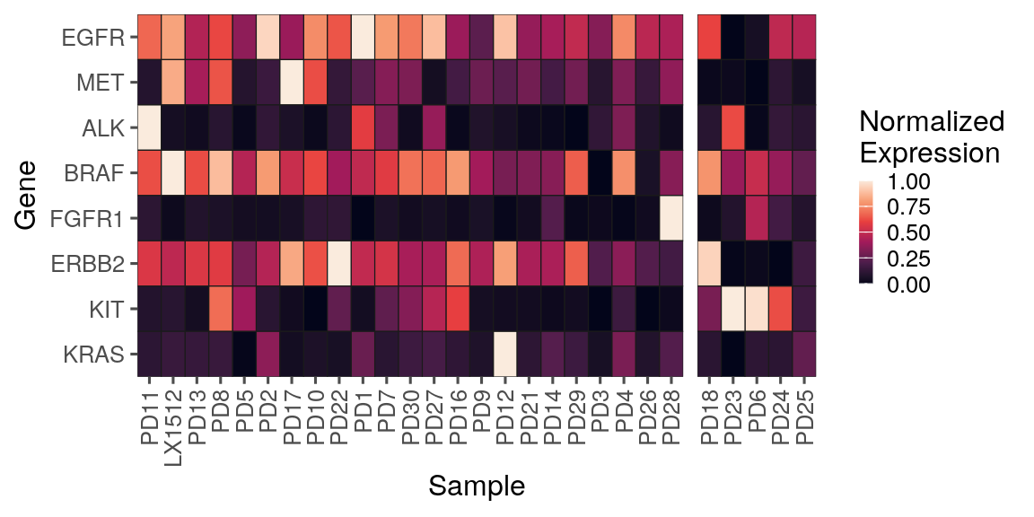
feats <- c("EGFR", "MET", "ALK", "BRAF", "FGFR1", "ERBB2", "KIT", "KRAS")
mapk_exp_df <- bulk_exp(srt_tum, cell_type_col = "is_tumor_cell", sample_id_col = "sample_id", meta_cols = c("time_point", "mapk_alt"), features = feats)

mapk_exp_df <- mapk_exp_df %>%
  filter(time_point == "PD", !is.na(mapk_alt)) %>%
  mutate(across(all_of(feats), ~ egfrnucseq::standardize(.x)))

mapk_exp_df_long <- mapk_exp_df %>%
  pivot_longer(cols = feats, names_to = "Gene", values_to = "exp")

p4 <- mapk_exp_df_long %>%
  ggplot(aes(x = fct_relevel(sample_id, samp_ord), y = as.numeric(fct_relevel(Gene, rev(names(gene_ord)))))) +
  geom_tile(aes(fill = exp), color = "grey10") +
  scale_fill_viridis_c(option = "rocket") +
  guides(
    x = guide_axis(angle = 90),
    fill = guide_colorbar(keywidth = 0.4, keyheight = 3)
  ) +
  # scale_y_discrete(expand = c(0,0)) +
  scale_y_continuous(
    expand = c(0, 0), breaks = 1:n_distinct(mapk_exp_df_long$Gene),
    labels = rev(unique(mapk_exp_df_long$Gene))
  ) +
  scale_x_discrete(expand = c(0, 0)) +
  theme_few() +
  theme(
    strip.text.x = element_blank(), strip.background.x = element_blank(), panel.border = element_blank()
  ) +
  facet_grid(. ~ mapk_alt, scales = "free", space = "free") +
  labs(x = "Sample", y = "Gene", fill = "Normalized\nExpression")
p4
```
```{r fig4e4f-mapk-alt-luad-sig-relapsed-plusmuts-plusexp, fig.width = 6, fig.height = 5.5}
pcomb <- (p1 + theme(plot.margin = margin())) + free(p2, type = "space", side = "b") + free((p3 + theme(plot.margin = margin(), axis.text.x = element_blank(), axis.ticks.x = element_blank(), axis.title.x = element_blank())), type = "space") + plot_spacer() + free(p4, type = "space") + plot_spacer() + plot_layout(ncol = 2, widths = c(1, 0.1), heights = c(1, 1, 0.6)) +
  plot_annotation(theme = theme(plot.margin = margin(3, 8, 15, 12, unit = "mm")))
ggsave(pcomb, file = here("plots", "mapk_alt_luad_sig_relapsed_plusmuts_plusexp.pdf"), width = 6, height = 5.5)

pcomb
```
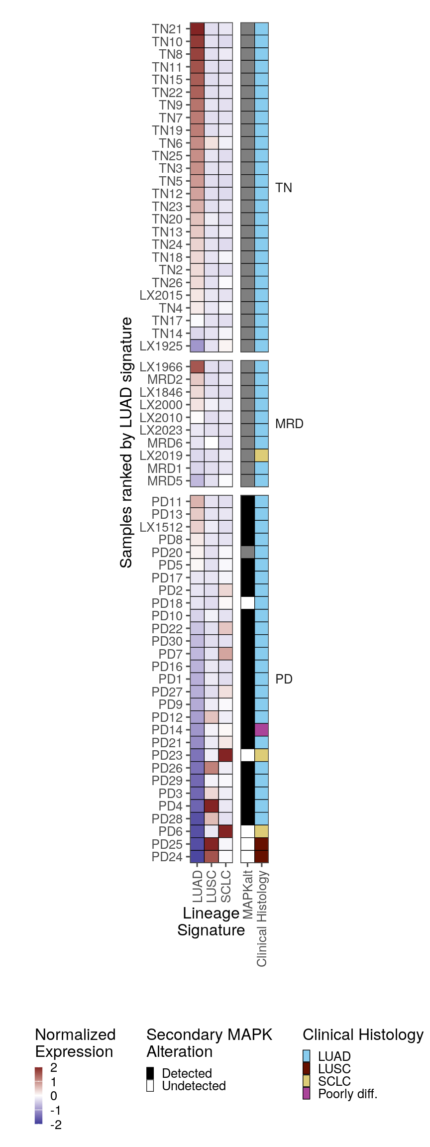
## Figure 4G -- lineage signature heatmap across specimens
Do the inverse test? Are samples identified with different histologies (i.e., LUSC and SCLC) were less likely to have an alternative MAPK-activating mutation (Fisher's exact test can be used for statistical support).
```{r}
feats <- c("LUAD", "LUSC", "SCLC")
sig_exp_df <- bulk_exp(srt_tum, cell_type_col = "is_tumor_cell", sample_id_col = "sample_id", meta_cols = c("time_point", "mapk_alt", "histology_predominant_short"), features = feats)

sig_exp_df <- sig_exp_df %>%
  # filter(time_point == "PD") %>%
  mutate(across(all_of(feats), ~ scale(.x)))

samp_ord2 <- fct_reorder(sig_exp_df$sample_id, -sig_exp_df$LUAD, median) %>%
  levels()

sig_exp_df_long <- sig_exp_df %>%
  pivot_longer(cols = feats, names_to = "Gene", values_to = "exp")

p0 <- sig_exp_df %>%
  ggplot(aes(x = fct_relevel(sample_id, samp_ord2))) +
  geom_tile(aes(y = "MAPKalt", fill = mapk_alt), show.legend = F, color = "black") +
  scale_fill_manual(
    values = c("MAPKalt" = "black", "Unknown" = "white"), breaks = c("MAPKalt"),
    labels = c("Secondary MAPK"), na.value = "white"
  ) +
  facet_grid(. ~ time_point, scales = "free", space = "free") +
  scale_x_discrete(expand = c(0, 0)) +
  scale_y_discrete(expand = c(0, 0)) +
  theme_few() +
  labs(y = NULL, x = NULL, fill = NULL) +
  theme(axis.text.x = element_blank(), axis.ticks.x = element_blank())

p1 <- sig_exp_df_long %>%
  ggplot(aes(x = fct_relevel(sample_id, samp_ord2), y = fct_relevel(Gene, "SCLC", "LUSC", "LUAD"))) +
  geom_tile(aes(fill = exp), color = "black") +
  # scale_fill_viridis_c(option = "rocket", oob = scales::squish, limits = c(-2, 2)) +
  scale_fill_gradient2(low = scales::muted("blue"), mid = "white", high = scales::muted("red"), oob = scales::squish, limits = c(-2, 2)) +
  facet_grid(. ~ time_point, scales = "free", space = "free") +
  scale_x_discrete(expand = c(0, 0)) +
  scale_y_discrete(expand = c(0, 0)) +
  labs(fill = "Normalized\nExpression", x = "Sample", y = "Lineage\nSignature") +
  guides(
    x = guide_axis(angle = 90),
    fill = guide_colorbar(keywidth = 0.4, keyheight = 3)
  ) +
  theme_few() +
  theme(strip.text.x = element_blank())
```
```{r fig4g-sig-heatmap-vertical, fig.width = 4.5, fig.height = 12}
library(ggpattern)

# sig_exp_df$secondary_mapk[sig_exp_df$sample_id %in% db$metadata$sample_id[!db$metadata$has_impact]] <- NA
p0 <- sig_exp_df %>%
  # mutate(secondary_mapk = ifelse(time_point %in% c("TN", "MRD"), "NA", secondary_mapk)) %>%
  ggplot(aes(x = fct_relevel(sample_id, rev(samp_ord2)))) +
  geom_tile(aes(y = "MAPKalt", fill = mapk_alt), show.legend = T, color = "black") +
  scale_fill_manual(
    name = "Secondary MAPK\nAlteration",
    values = c("MAPKalt" = "black", "Unknown" = "white", "NA" = "grey60"), breaks = c("MAPKalt", "Unknown", "NA"),
    labels = c("Detected", "Undetected", "Not applicable")
  ) +
  guides(fill = guide_legend(keywidth = 0.4, keyheight = 0.5, order = 1)) +
  ggnewscale::new_scale_fill() +
  geom_tile(aes(y = "Clinical Histology", fill = histology_predominant_short), color = "black") +
  scale_fill_manual(
    name = "Clinical Histology", values = colors$histology_predominant_short,
    breaks = names(colors$histology_predominant_short)
  ) +
  guides(fill = guide_legend(keywidth = 0.4, keyheight = 0.5, order = 2)) +
  facet_grid(time_point ~ ., scales = "free", space = "free") +
  scale_x_discrete(expand = c(0, 0)) +
  scale_y_discrete(expand = c(0, 0), limits = c("MAPKalt", "Clinical Histology")) +
  guides(x = guide_axis(angle = 90)) +
  theme_few() +
  labs(y = NULL, x = NULL, fill = NULL) +
  theme(
    axis.text.y = element_blank(), axis.ticks.y = element_blank(),
    strip.text.y.right = element_text(angle = 0, hjust = 0)
  ) +
  coord_flip()

p1 <- sig_exp_df_long %>%
  ggplot(aes(x = fct_relevel(sample_id, rev(samp_ord2)), y = fct_relevel(Gene, "LUAD", "LUSC", "SCLC"))) +
  geom_tile(aes(fill = exp), color = "black") +
  # scale_fill_viridis_c(option = "rocket", oob = scales::squish, limits = c(-2, 2)) +
  scale_fill_gradient2(low = scales::muted("blue"), mid = "white", high = scales::muted("red"), oob = scales::squish, limits = c(-2, 2)) +
  facet_grid(time_point ~ ., scales = "free", space = "free") +
  scale_x_discrete(expand = c(0, 0)) +
  scale_y_discrete(expand = c(0, 0)) +
  labs(fill = "Normalized\nExpression", x = "Samples ranked by LUAD signature", y = "Lineage\nSignature") +
  guides(
    x = guide_axis(angle = 90),
    fill = guide_colorbar(keywidth = 0.4, keyheight = 3)
  ) +
  theme_few() +
  theme(strip.text.y = element_blank()) +
  coord_flip()

pcomb <- free((p1 + theme(plot.margin = margin(4, 2, 0, 30, "mm"))), type = "label", side = "b") + (p0 + theme(plot.margin = margin(4, 30, 2, 0, "mm"))) + plot_layout(ncol = 2, widths = c(1, 0.66), guides = "collect") + plot_annotation(theme = theme(legend.position = "bottom", legend.box.margin = margin(), legend.margin = margin()))

pcomb
ggsave(pcomb, file = here("plots", "sig_heatmap_vertical.pdf"), width = 4.5, height = 12)
```
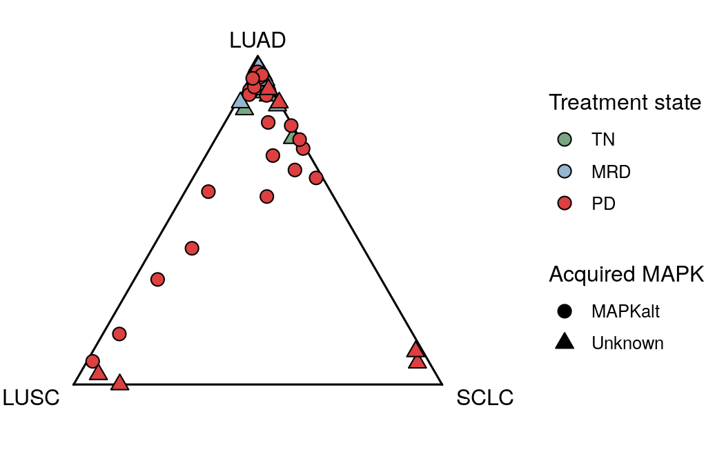
## Figure 4I -- ternary diagram of histological signatures
```{r fig4i-sample-ternary-mapk, fig.width = 5.4, fig.height = 3.4}
sig_exp_df <- bulk_exp(srt_tum, cell_type_col = "is_tumor_cell", sample_id_col = "sample_id", meta_cols = c("time_point", "mapk_alt"), features = c("LUAD", "LUSC", "SCLC"))

# devtools::load_all()
sig_exp_df <- sig_exp_df %>%
  # filter(time_point == "PD") %>%
  mutate(across(all_of(c("LUAD", "LUSC", "SCLC")), ~ egfrnucseq::standardize(.x)))

sig_exp_df$mapk_alt[is.na(sig_exp_df$mapk_alt)] <- "Unknown"
# sig_exp_df$secondary_mapk[sig_exp_df$time == "Pre"] <- "N/A"

library(ggtern)

p1 <- sig_exp_df %>%
  mutate(acquired_mapk = ifelse(mapk_alt == "MAPKalt", "MAPKalt", "Unknown")) %>%
  ggtern(aes(y = LUAD, x = LUSC, z = SCLC)) +
  geom_mask() +
  geom_point(aes(fill = time_point, shape = acquired_mapk), size = 3, show.legend = T) +
  scale_fill_manual(values = colors$time_point) +
  scale_shape_manual(values = c(21, 24)) +
  theme_classic() +
  Tlab("LUAD") + Llab("LUSC") + Rlab("SCLC") +
  theme_nolabels() +
  # theme_nomask() +
  guides(
    fill = guide_legend(override.aes = list(shape = 21)),
    shape = guide_legend(override.aes = list(fill = "black"))
  ) +
  labs(fill = "Treatment state", shape = "Acquired MAPK") +
  theme_noticks() +
  theme(panel.background = element_blank(), panel.border = element_blank()) +
  # facet_grid(.~time_point, switch = "x") +
  theme(
    # axis.title = element_markdown(color = "blue"), # This is where to do it
    strip.background = element_part_rect(side = ""),
    legend.position = "right",
    strip.text.x.bottom = element_text(size = 12, face = "bold")
  )
ggsave(p1, file = here("plots", "sample_ternary_mapk.pdf"), width = 5.4, height = 3.4)
p1
detach("package:ggtern", unload = TRUE)
```
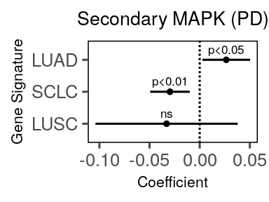
## Figure 4J -- MAPKalt association with each histological signature
Look at EGFR and MAPK mapk pathway in PD transformed vs not
Do a model with MAPKalt vs not for the three histologies, then a model for each mutation's association with LUSC and SCLC
```{r}
# library(lme4)
library(tidyr)
library(broom.mixed)

dat <- srt_tum@meta.data %>%
  filter(time_point == "PD", !is.na(mapk_alt)) %>%
  group_by(sample_id, mapk_alt, time_point) %>%
  summarize(across(c(LUAD, LUSC, SCLC), mean)) %>%
  mutate(mapk_alt = factor(mapk_alt, levels = c("Unknown", "MAPKalt")))

mods <- map(c("LUAD", "LUSC", "SCLC"), .f = function(pth) {
  mod <- lm(glue::glue("{pth} ~ mapk_alt"), dat) %>%
    broom::tidy(conf.int = TRUE) %>%
    mutate(Signature = pth, .before = 1) %>%
    filter(term == "mapk_altMAPKalt")
}) %>%
  list_rbind()

mods <- mods %>%
  rstatix::add_significance(
    p.col = "p.value",
    cutpoints = c(0, 1e-04, 0.001, 0.01, 0.05, 0.1, 1),
    symbols = c("p<0.0001", "p<0.001", "p<0.01", "p<0.05", "p<0.1", "ns")
  )
```
```{r fig4j-acquired-mapk-lm, fig.width = 2, fig.height = 1.5}
p <- mods %>%
  ggplot(., aes(x = estimate, y = fct_reorder(Signature, estimate, mean))) +
  geom_pointrange(aes(x = estimate, xmin = conf.low, xmax = conf.high), fatten = 0.4) +
  geom_vline(xintercept = 0, linetype = "11") +
  theme_few() +
  theme(
    axis.line = element_blank(),
    panel.border = element_rect(fill = NA, color = "black"),
    strip.background = element_blank(),
    plot.title = element_text(size = 10, hjust = 0.5),
    axis.title = element_text(size = 8)
  ) +
  labs(y = "Gene Signature", x = "Coefficient", title = "Secondary MAPK (PD)") +
  geom_text(data = {
    filter(mods, p.value != "ns")
  }, aes(y = Signature, x = estimate, label = p.value.signif), nudge_y = 0.325, size = 2.25)
ggsave(p, file = here("plots", "acquired_mapk_lm.pdf"), width = 2, height = 1.5)
p
```
# Figure S9 -- Lineage signatures and MAPK pathway activity
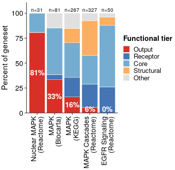
## Figure S9A -- functional-tier composition of the MAPK gene sets
Functional-tier composition of the same five gene sets. The overlap views above show
*which* genes the sets share; this shows *what kind* of genes each one is made of, and
is what licenses using Nuclear MAPK (Reactome) as the pathway-output readout
throughout Figure 4 -- it is 81% Output-tier, against 0% for EGFR Signaling.
Tier assignments are curated in `paper_data/annotated_gene_table_final.csv` (Table S6);
see STAR Methods, "Functional-tier classification of MAPK pathway gene-set members".
```{r figs9a-mapk-tier-composition, fig.width = 1.85, fig.height = 1.8}
annot_tiers <- read.csv(here("paper_data", "annotated_gene_table_final.csv"))

# membership column -> display name (exact names as used in the paper)
sets_map <- c(
  REACTOME_MAPK_TARGETS_NUCLEAR_EVENTS_MEDIATED_BY_MAP_KINASES = "Nuclear MAPK (Reactome)",
  REACTOME_MAPK_FAMILY_SIGNALING_CASCADES                      = "MAPK Cascades (Reactome)",
  REACTOME_SIGNALING_BY_EGFR                                   = "EGFR Signaling (Reactome)",
  KEGG_MAPK_SIGNALING_PATHWAY                                  = "MAPK (KEGG)",
  BIOCARTA_MAPK_PATHWAY                                        = "MAPK (Biocarta)"
)

tier_lv <- c("Output", "Receptor", "Core", "Structural", "Other")

stopifnot(
  all(names(sets_map) %in% colnames(annot_tiers)),
  "functional_tier" %in% colnames(annot_tiers),
  all(annot_tiers$functional_tier %in% tier_lv)
)

comp <- imap_dfr(sets_map, function(display, col) {
  genes <- annot_tiers %>% filter(.data[[col]] == 1)
  tibble(set = display, tier = genes$functional_tier) %>%
    dplyr::count(set, tier, name = "n") %>%
    mutate(pct = 100 * n / sum(n), total = nrow(genes))
}) %>%
  complete(set, tier = tier_lv, fill = list(n = 0, pct = 0)) %>%
  group_by(set) %>% fill(total, .direction = "downup") %>% ungroup()

# Sets ordered left-to-right by decreasing Output content
tier_ord <- comp %>% filter(tier == "Output") %>% arrange(dplyr::desc(pct)) %>% pull(set)
tier_lab <- setNames(sub(" \\(", "\n(", tier_ord), tier_ord)
tier_pal <- c(Output = "#d73027", Receptor = "#4575b4", Core = "#74add1",
              Structural = "#fdae61", Other = "#e0e0e0")

d_tier <- comp %>% mutate(set = factor(set, levels = tier_ord),
                          tier = factor(tier, levels = rev(tier_lv)))
outlab <- comp %>% filter(tier == "Output") %>%
  mutate(set = factor(set, levels = tier_ord),
         y = ifelse(pct >= 12, pct / 2, 4), txt = sprintf("%.0f%%", pct))
ntop <- comp %>% distinct(set, total) %>%
  mutate(set = factor(set, levels = tier_ord), txt = sprintf("n=%d", total))

p_tier <- ggplot(d_tier, aes(set, pct, fill = tier)) +
  geom_col(width = 0.9, colour = "white", linewidth = 0.1) +
  geom_text(data = outlab, aes(set, y, label = txt), inherit.aes = FALSE,
            colour = "white", size = 2.0, fontface = "bold") +
  geom_text(data = ntop, aes(set, 101.5, label = txt), inherit.aes = FALSE,
            size = 1.35, vjust = 0, colour = "black") +
  scale_fill_manual(values = tier_pal, breaks = tier_lv, name = "Functional tier") +
  scale_x_discrete(labels = tier_lab) +
  scale_y_continuous(expand = expansion(mult = c(0, 0.09))) +
  labs(x = NULL, y = "Percent of geneset") +
  guides(fill = guide_legend(ncol = 1, title.position = "top",
                             keyheight = unit(0.18, "cm"),
                             keywidth  = unit(0.18, "cm"))) +
  theme_classic(base_size = 6) +
  theme(
    axis.text.x  = element_text(size = 5.2, angle = 90, hjust = 1, vjust = 0.5,
                                colour = "black", lineheight = 0.85),
    axis.text.y  = element_text(size = 5.4, colour = "black"),
    axis.title.y = element_text(size = 5.8),
    axis.ticks   = element_line(linewidth = 0.16),
    axis.line    = element_line(linewidth = 0.16),
    legend.title = element_text(size = 5.4, face = "bold"),
    legend.text  = element_text(size = 5.0),
    legend.position      = "right",
    legend.key.spacing.y = unit(0.3, "pt"),
    legend.margin        = margin(0, 0, 0, 1),
    legend.box.spacing   = unit(3, "pt"),
    plot.margin          = margin(2, 2, 1, 1)
  )

# device = "pdf" (base), NOT cairo_pdf -- cairo compresses word spacing in the
# rotated x-axis labels.
ggsave(here("plots", "mapk_tier_composition.pdf"), p_tier,
       width = 1.85, height = 1.8, device = "pdf")
p_tier
```
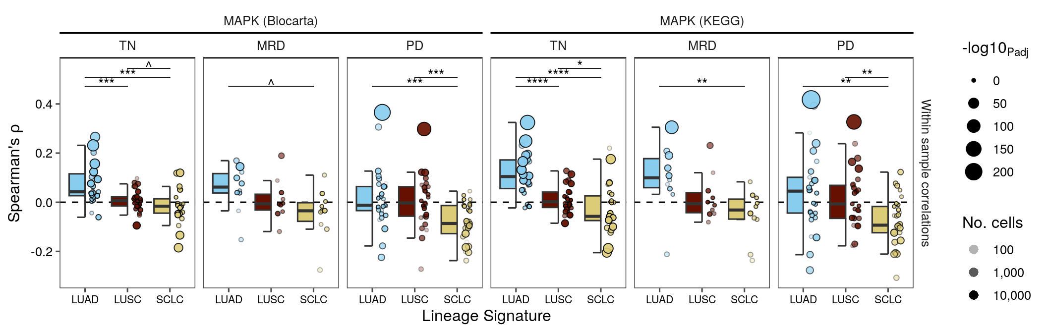
## Figure S9B -- within-specimen Biocarta and KEGG MAPK correlations
```{r figs9b-per-sample-mapk-cor-supp, fig.width = 11, fig.height = 3.5}
p <- per_sample_cor %>%
  filter(Parameter2 != "REACTOME_MAPK_TARGETS_NUCLEAR_EVENTS_MEDIATED_BY_MAP_KINASES") %>%
  arrange(desc(p)) %>%
  ggplot(aes(x = Parameter1, y = rho)) +
  geom_hline(yintercept = 0, linetype = "dashed") +
  gghalves::geom_half_boxplot(outliers = F, aes(fill = Parameter1),
                               errorbar.draw = T) +
  gghalves::geom_half_point_panel(aes(size = -log10(p), fill = Parameter1,
                                      alpha = n_Obs),
                                  transformation = position_jitter(width = 0.5), pch = 21) +
  facet_nested("Within sample correlations" ~ mapk_path + time_point) +
  scale_fill_manual(values = colors$histology_predominant_short) +
  scale_alpha_continuous(trans = "log10", breaks = scales::breaks_log(), labels = scales::label_number(big.mark = ",")) +
  guides(
    fill = "none",
    x = guide_axis(angle = 0),
    size = guide_legend(override.aes = list(pch = 19)),
    alpha = guide_legend(override.aes = list(pch = 16, size = 3))
  ) +
  ggpubr::geom_pwc(tip.length = 0, label = "p.adj.signif", step.increase = 0.05, vjust = 0.5, hide.ns = T, bracket.nudge.y = 0.075, symnum.args = symnum_0.1_star) +
  theme_few() +
  theme(
    strip.background.x = element_part_rect(side = "b", fill = NA, color = "black"),
    strip.clip = "off",
    plot.title = element_text(hjust = 0.5, size = 12), plot.title.position = "panel",
    axis.text = element_text(color = "black"),
    axis.text.x = element_text(size = 8)
  ) +
  labs(x = "Lineage Signature", y = bquote("Spearman's" ~ rho), size = bquote("-log10"[Padj]), alpha = "No. cells")
ggsave(p, file = here("plots", "per_sample_mapk_cor_supp.pdf"), width = 11, height = 3.5)
p
```
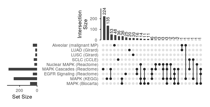
## Figure S9E -- gene-membership overlap among lineage and MAPK sets
```{r, fig.width = 5, fig,height = 4}
plist <- split(pathways_v2$Gene, pathways_v2$pathway)

meta_programs_df <- read.table(file = "https://raw.githubusercontent.com/mjz1/meta_programs_tirosh/refs/heads/main/tirosh_mp_patched.txt", header = T, sep = "\t")

meta_programs <- split(meta_programs_df, meta_programs_df$cell_type)

meta_programs <- map(meta_programs, .f = function(x) {
  res <- split(x, x$meta_program)
  map(res, .f = function(y) y$Gene)
})

names(meta_programs) <- janitor::make_clean_names(names(meta_programs))
```
```{r figs9e-mapk-path-overlaps-upset, fig.width = 3.6, fig.height = 1.85}
# UpSet over all five core MAPK pathways (the Euler stays trimmed). Hand-rolled in
# ggplot2 + patchwork because ComplexUpset is incompatible with ggplot2 4.x and UpSetR
# strands its "Intersection Size" axis title far from its axis.
library(tidyverse)
library(patchwork)

upset_sel <- list(
  "Alveolar (malignant MP)"  = meta_programs$malignant$alveolar,
  "LUAD (Girard)"            = plist$LUAD_GIRARD,
  "LUSC (Girard)"            = plist$LUSC_GIRARD,
  "SCLC (CCLE)"              = plist$SCLC_CCLE,
  "Nuclear MAPK (Reactome)"  = plist$REACTOME_MAPK_TARGETS_NUCLEAR_EVENTS_MEDIATED_BY_MAP_KINASES,
  "MAPK Cascades (Reactome)" = plist$REACTOME_MAPK_FAMILY_SIGNALING_CASCADES,
  "EGFR Signaling (Reactome)"= plist$REACTOME_SIGNALING_BY_EGFR,
  "MAPK (KEGG)"              = plist$KEGG_MAPK_SIGNALING_PATHWAY,
  "MAPK (Biocarta)"          = plist$BIOCARTA_MAPK_PATHWAY
)
upset_sel <- purrr::map(upset_sel, unique)

# Build an UpSet (exclusive intersections, like UpSetR's default) from a named
# list of sets. `min_size` drops empty combinations; `n_max` caps the number of
# intersection bars (set to a number, e.g. 25, if the plot gets too busy).
# Namespaces are explicit (dplyr::/tidyr::) to avoid masking by other attached
# packages in this qmd (e.g. count/filter/slice).
upset_gg <- function(sel, min_size = 1, n_max = Inf, dot = 1.1, base_size = 6.5) {
  sets  <- names(sel)
  genes <- unique(unlist(sel))
  mat   <- vapply(sel, function(s) genes %in% s, logical(length(genes)))
  # Each gene's "combo" = the exact set of sets it belongs to.
  key   <- apply(mat, 1, function(r) paste(which(r), collapse = ","))
  combo_df <- tibble::tibble(key = key) |>
    dplyr::filter(key != "") |>
    dplyr::count(key, name = "size") |>
    dplyr::filter(size >= min_size) |>
    dplyr::arrange(dplyr::desc(size)) |>
    dplyr::slice_head(n = n_max) |>
    dplyr::mutate(combo_id = dplyr::row_number())

  set_lv  <- rev(sets)  # first set on top
  mat_df  <- combo_df |>
    dplyr::mutate(set_idx = strsplit(key, ",")) |>
    tidyr::unnest(set_idx) |>
    dplyr::mutate(set = factor(sets[as.integer(set_idx)], levels = set_lv))
  grid_df <- tidyr::expand_grid(combo_id = combo_df$combo_id, set = factor(sets, levels = set_lv))
  size_df <- tibble::tibble(set = factor(sets, levels = set_lv), size = colSums(mat))

  xexp <- expansion(add = 0.6)
  base <- theme_minimal(base_size = base_size) +
    theme(panel.grid = element_blank())
  axis_ln <- element_line(linewidth = 0.3)

  p_top <- ggplot(combo_df, aes(combo_id, size)) +
    geom_col(width = 0.6, fill = "grey25") +
    # Counts rotated vertical so they never collide horizontally — this is what
    # lets the figure shrink. The tall counts (224/135) need headroom that
    # scales with the (short) bar panel: generous top expansion plus clip = off
    # and a top margin keep them from being cut at the device edge.
    geom_text(aes(label = size), angle = 90, hjust = -0.2, vjust = 0.5, size = 1.8) +
    scale_x_continuous(expand = xexp) +
    scale_y_continuous("Intersection\nSize", expand = expansion(mult = c(0, 0.33)),
                       breaks = scales::breaks_extended(4)) +
    coord_cartesian(clip = "off") +
    base + theme(axis.title.x = element_blank(), axis.text.x = element_blank(),
                 axis.ticks.x = element_blank(),
                 axis.line.y = axis_ln, axis.ticks.y = axis_ln,
                 plot.margin = margin(t = 5, r = 2, b = 1, l = 1))

  p_mat <- ggplot(mapping = aes(combo_id, set)) +
    geom_point(data = grid_df, color = "grey88", size = dot) +
    geom_line(data = mat_df, aes(group = combo_id), linewidth = 0.4, color = "grey20") +
    geom_point(data = mat_df, color = "grey15", size = dot) +
    scale_x_continuous(expand = xexp) +
    scale_y_discrete(expand = expansion(add = 0.4)) +
    base + theme(axis.title = element_blank(), axis.text.x = element_blank(),
                 axis.ticks = element_blank())

  p_left <- ggplot(size_df, aes(size, set)) +
    geom_col(width = 0.6, fill = "grey25") +
    scale_x_reverse("Set Size", expand = expansion(mult = c(0.05, 0)),
                    breaks = scales::breaks_extended(3)) +
    scale_y_discrete(expand = expansion(add = 0.4)) +
    base + theme(axis.title.y = element_blank(), axis.text.y = element_blank(),
                 axis.line.x = axis_ln, axis.ticks.x = axis_ln,
                 axis.ticks.y = element_blank())

  # Grid: top bars over the matrix (shared x); set-size bars left of the matrix
  # (shared y). patchwork aligns the shared panel edges automatically.
  # free(type = "space", side = "l") stops the top plot from reserving the wide
  # gutter needed by the matrix's long set-name labels, so the "Intersection
  # Size" title sits flush against its own axis instead of drifting left.
  patchwork::free(p_top, type = "space", side = "l") + p_left + p_mat +
    plot_layout(design = "#A\nBC", widths = c(1, 3.4), heights = c(1.5, 2.0))
}

# 3.6 x 1.85 in is about the smallest legible footprint for these 27
# intersections: below ~3.4 wide the dot columns / size-1 tail crowd, and below
# ~1.75 tall the set-name labels collide.
p_upset <- upset_gg(upset_sel, min_size = 1)
ggsave(here("plots", "mapk_path_overlaps_upset.pdf"), p_upset, width = 3.6, height = 1.85)
p_upset
```
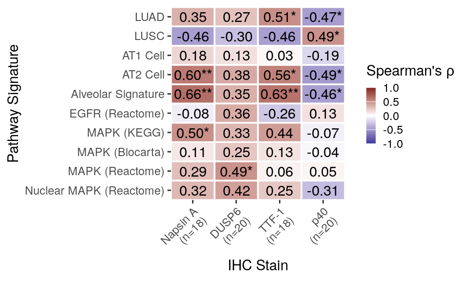
## Figure S9F -- signature vs IHC H-score correlation matrix
The IHC x pathway correlation the panel below plots.
Correlate with summarized signatures
```{r}
paths <- unique(c(pathways$pathway, pathways_v2$pathway, grep("^mp", colnames(srt_tum@meta.data), value = T)))

sig_exp_df <- bulk_exp(srt_tum, cell_type_col = "is_tumor_cell", sample_id_col = "sample_id", meta_cols = c("time_point", "mapk_alt"), features = paths)

# `mapk_alt` is the literal string "NA" on the object where Table S1 has a real NA, so a
# natural join on the shared columns drops every TN and MRD specimen. Key on sample_id.
ihc_ <- ihc_long %>%
  filter(sample_id %in% unique(srt_tum$sample_id)) %>%
  pivot_wider(id_cols = c("sample_id", "time_point", "mapk_alt"), names_from = stain, values_from = value) %>%
  inner_join(dplyr::select(sig_exp_df, -dplyr::any_of(c("time_point", "mapk_alt"))),
             by = "sample_id") %>%
  ungroup()

# The n= in the axis labels is counted off `ihc_`, so a lossy join would understate it
# silently rather than error.
stopifnot(nrow(ihc_) == length(intersect(as.character(unique(ihc_long$sample_id)),
                                         as.character(sig_exp_df$sample_id))))

# res_full <- correlation::correlation(ihc_, select = "erk_ph_nuclear", select2 = paths, method = "spearman", p_adjust = "none")

select_paths <- c("LUAD", "LUSC", grep("EGFR|MAPK|ALVEOLAR", ignore.case = T, paths, value = T))

select_stains <- c("napsin_a_cytoplasmic", "dusp6_cytoplasmic", "ttf_1_nuclear", "p40_nuclear")
# select_stains <- unique(df$stain)

# Filter to keep only pathways related to lung tumor alveolar biology or EGFR signaling
# Names match Figure 3C sig_heatmap convention
pathway_names <- c(
  "LUAD" = "LUAD",
  "LUSC" = "LUSC",
  "TRAVAGLINI_LUNG_ALVEOLAR_EPITHELIAL_TYPE_1_CELL" = "AT1 Cell",
  "TRAVAGLINI_LUNG_ALVEOLAR_EPITHELIAL_TYPE_2_CELL" = "AT2 Cell",
  "mp44_alveolar" = "Alveolar Signature",
  "REACTOME_SIGNALING_BY_EGFR" = "EGFR (Reactome)",
  "KEGG_MAPK_SIGNALING_PATHWAY" = "MAPK (KEGG)",
  "BIOCARTA_MAPK_PATHWAY" = "MAPK (Biocarta)",
  "REACTOME_MAPK_FAMILY_SIGNALING_CASCADES" = "MAPK (Reactome)",
  # "REACTOME_ONCOGENIC_MAPK_SIGNALING" = "Oncogenic MAPK Signaling (Reactome)",
  "REACTOME_MAPK_TARGETS_NUCLEAR_EVENTS_MEDIATED_BY_MAP_KINASES" = "Nuclear MAPK (Reactome)"
)

stain_rename <- c(
  "napsin_a_cytoplasmic" = "Napsin A",
  "dusp6_cytoplasmic" = "DUSP6",
  "ttf_1_nuclear" = "TTF-1",
  "p40_nuclear" = "p40"
)

# Count number of samples with a non-missing value for each stain and append
# to the display name so sample sizes are visible on the x-axis
stain_n <- sapply(names(stain_rename), function(col) sum(!is.na(ihc_[[col]])))
stain_rename <- setNames(glue("{stain_rename}\n(n={stain_n})"), names(stain_rename))

ihc_rename <- ihc_ %>%
  rename_with(~ recode(., !!!pathway_names), .cols = all_of(names(pathway_names))) %>%
  rename_with(~ recode(., !!!stain_rename), .cols = all_of(names(stain_rename)))

res <- correlation::correlation(ihc_rename, select = pathway_names, select2 = stain_rename, method = "spearman", p_adjust = "none")

library(correlation); library(see)

s <- summary(res)
```
```{r figs9f-ihc-pathway-correlation, fig.width = 5, fig.height = 3}
p <- plot(s) +
  guides(x = guide_axis(angle = 45)) +
  scale_fill_gradient2(low = scales::muted("blue"), mid = "white", high = scales::muted("red"), midpoint = 0, limits = c(-1, 1)) +
  labs(y = "Pathway Signature",
       x = "IHC Stain",
       title = NULL,
       fill = bquote("Spearman's" ~ rho)) +
  guides(fill = guide_colorbar(keywidth = 0.5, keyheight = 3))
p
ggsave(p, file = here("plots", "ihc_pathway_correlation.pdf"), width = 5, height = 3)
```