---
title: "LuCA Atlas Analysis"
author: "Matthew Zatzman"
date: "`r Sys.Date()`"
execute:
warning: false
error: false
format:
html:
code-fold: true
code-tools: true
toc: true
---
Reproduces Figures 4C-D, S7C and S9C from the LuCA atlas deposit.
```{r setup}
#| output: false
library(tidyverse)
library(here)
library(ggbeeswarm)
library(ggthemes)
library(ggh4x)
library(glue)
library(patchwork)
library(Seurat)
devtools::load_all()
# stat_cor() pastes the p value in as a double, so its notation follows `scipen`. The
# published panels were rendered at R's default of 0 -- Fig 4C reads "p = 2e-05". A
# session that picked up a personal ~/.Rprofile setting scipen > 0 renders "p = 0.00002"
# instead, silently diverging from the paper.
options(scipen = 0)

markers <- load_markers()

symnum_0.1 <- list(cutpoints = c(0, 1e-04, 0.001, 0.01, 0.05, 0.1, Inf), symbols = c(
  "p<0.0001",
  "p<0.001", "p<0.01", "p<0.05", "p<0.1", "ns"
))
```
# Load Data
```{r}
luca <- readRDS(here("paper_data", "luca_extended.rds"))

luca <- luca[, luca$ann_coarse == "Epithelial cell"]

scores <- read.table(file = here("paper_data", "luca_ucell_signatures.txt.gz"), header = T, sep = "\t")
rownames(scores) <- scores$cell_id
scores$cell_id <- NULL
luca <- AddMetaData(luca, scores)
```
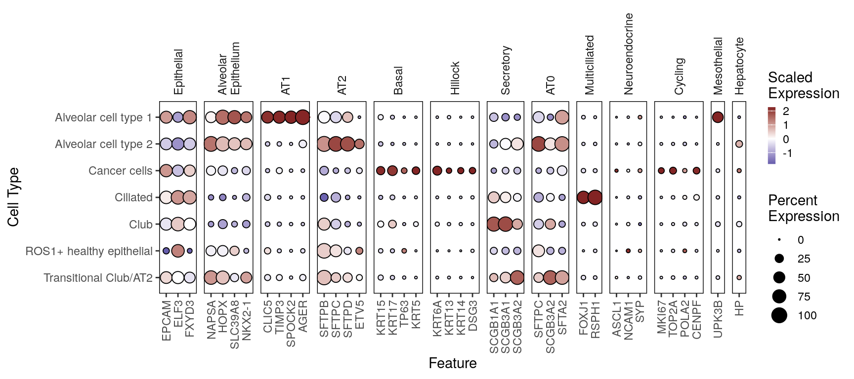
# Check Markers
```{r, fig.width = 9, fig.height = 4}
#| warning: false
p <- DotPlotter(luca, features = markers$epi_markers_final, group.by = "ann_fine", rotate_y_strip = T)
p
```
# Compute mean scores and plot
```{r}
sample_df <- luca@meta.data %>%
  add_count(sample, name = "n_epi") %>%
  add_count(sample, ann_fine, name = "n_fine") %>%
  mutate(prop_fine = n_epi / n_fine) %>%
  select(study, dataset, donor_id, sample, origin, platform, n_epi, ends_with("_mutation")) %>%
  distinct()

mean_scores <- luca@meta.data %>%
  group_by(sample) %>%
  add_count(name = "n_samp") %>%
  filter(n_samp >= 100) %>%
  group_by(study, disease, dataset, donor_id, sample, origin, platform, ann_fine, tumor_stage, uicc_stage) %>%
  add_count(name = "n_fine") %>%
  filter(n_fine >= 20) %>%
  summarize(across(colnames(scores), ~ mean(.x, na.rm = T))) %>%
  ungroup() %>%
  left_join(select(sample_df, sample, ends_with("_mutation")))

mean_scores_long <- mean_scores %>%
  pivot_longer(cols = colnames(scores), names_to = "Pathway", values_to = "mean_exp")
```
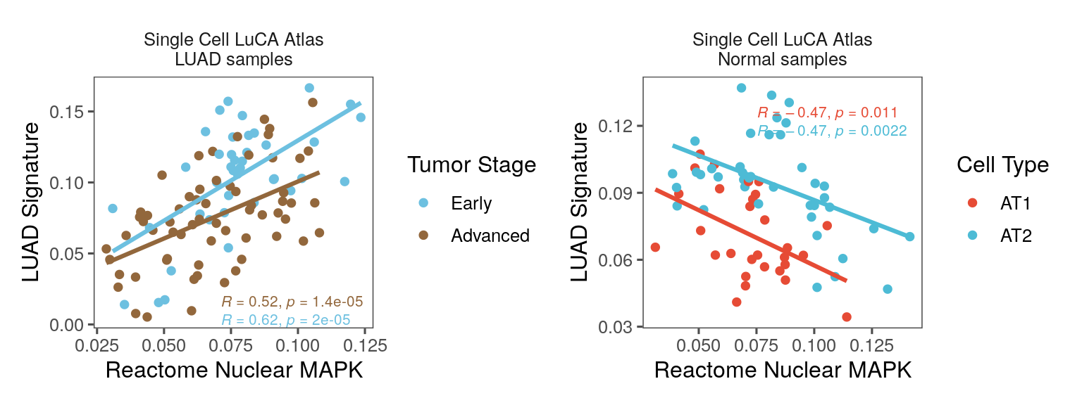
# Figure 4C-D -- nuclear MAPK versus LUAD identity
<!-- panels: 4C-D -->
```{r, fig.width = 8, fig.height = 3}
# Six `normal_adjacent` samples also carry a cancer-cell call; excluding them is what makes
# this the 103 tumor samples (91 patients) the published panel reports.
df <- mean_scores %>%
  filter(ann_fine == "Cancer cells" & disease %in% c("lung adenocarcinoma") & origin != "normal_adjacent")

stopifnot(nrow(df) == 103)

p1 <- df %>%
  ggplot(aes(x = REACTOME_MAPK_TARGETS_NUCLEAR_EVENTS_MEDIATED_BY_MAP_KINASES, y = LUAD_GIRARD, color = tumor_stage)) +
  geom_point() +
  geom_smooth(method = "lm", show.legend = F, se = F) +
  ggpubr::stat_cor(show.legend = F, size = 2.75, label.x.npc = 0.45, label.y.npc = 0.075) +
  facet_grid(. ~ glue("Single Cell LuCA Atlas\nLUAD samples")) +
  see::scale_color_bluebrown_d(reverse = T, breaks = c("early", "advanced"), labels = c("Early", "Advanced")) +
  theme_few() +
  labs(x = "Reactome Nuclear MAPK", y = "LUAD Signature", color = "Tumor Stage")


df2 <- mean_scores %>%
  filter(ann_fine %in% c("Alveolar cell type 1", "Alveolar cell type 2") & origin %in% c("normal"))

# 29 AT1 and 40 AT2 per-sample profiles, from 45 normal samples.
stopifnot(nrow(df2) == 69)

p2 <- df2 %>%
  ggplot(aes(x = REACTOME_MAPK_TARGETS_NUCLEAR_EVENTS_MEDIATED_BY_MAP_KINASES, y = LUAD_GIRARD, color = ann_fine)) +
  geom_point() +
  geom_smooth(method = "lm", show.legend = F, se = F) +
  ggpubr::stat_cor(show.legend = F, size = 2.75, label.x.npc = 0.4, label.y.npc = 0.9) +
  facet_grid(. ~ glue("Single Cell LuCA Atlas\nNormal samples")) +
  scale_color_manual(values = c("#E64B35FF", "#4DBBD5FF"), breaks = c("Alveolar cell type 1", "Alveolar cell type 2"), labels = c("AT1", "AT2")) +
  theme_few() +
  labs(x = "Reactome Nuclear MAPK", y = "LUAD Signature", color = "Cell Type")

pcomb <- p1 | p2
ggsave(pcomb, file = here("plots", "luca_atlas_mapk_cor_plus_norm.pdf"), width = 8, height = 3)
pcomb
```
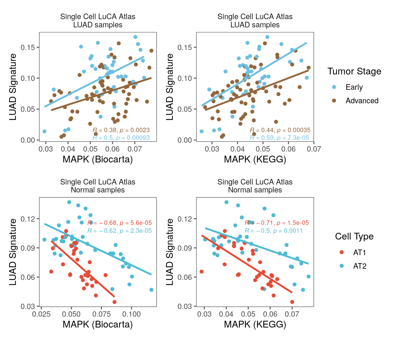
# Figure S9C -- Biocarta and KEGG MAPK versus LUAD identity
<!-- panels: S9C -->
The same tumor and normal comparisons as 4C-D, repeated for the two other MAPK gene sets.
```{r, fig.width = 7, fig.height = 6}
p1 <- df %>%
  ggplot(aes(x = BIOCARTA_MAPK_PATHWAY, y = LUAD_GIRARD, color = tumor_stage)) +
  geom_point() +
  geom_smooth(method = "lm", show.legend = F, se = F) +
  ggpubr::stat_cor(show.legend = F, size = 2.75, label.x.npc = 0.45, label.y.npc = 0.075) +
  facet_grid(. ~ glue("Single Cell LuCA Atlas\nLUAD samples")) +
  see::scale_color_bluebrown_d(reverse = T, breaks = c("early", "advanced"), labels = c("Early", "Advanced")) +
  theme_few() +
  labs(x = "MAPK (Biocarta)", y = "LUAD Signature", color = "Tumor Stage")

p2 <- df2 %>%
  ggplot(aes(x = BIOCARTA_MAPK_PATHWAY, y = LUAD_GIRARD, color = ann_fine)) +
  geom_point() +
  geom_smooth(method = "lm", show.legend = F, se = F) +
  ggpubr::stat_cor(show.legend = F, size = 2.75, label.x.npc = 0.4, label.y.npc = 0.8) +
  facet_grid(. ~ glue("Single Cell LuCA Atlas\nNormal samples")) +
  scale_color_manual(values = c("#E64B35FF", "#4DBBD5FF"), breaks = c("Alveolar cell type 1", "Alveolar cell type 2"), labels = c("AT1", "AT2")) +
  theme_few() +
  labs(x = "MAPK (Biocarta)", y = "LUAD Signature", color = "Cell Type")

p3 <- df %>%
  ggplot(aes(x = KEGG_MAPK_SIGNALING_PATHWAY, y = LUAD_GIRARD, color = tumor_stage)) +
  geom_point() +
  geom_smooth(method = "lm", show.legend = F, se = F) +
  ggpubr::stat_cor(show.legend = F, size = 2.75, label.x.npc = 0.45, label.y.npc = 0.075) +
  facet_grid(. ~ glue("Single Cell LuCA Atlas\nLUAD samples")) +
  see::scale_color_bluebrown_d(reverse = T, breaks = c("early", "advanced"), labels = c("Early", "Advanced")) +
  theme_few() +
  labs(x = "MAPK (KEGG)", y = "LUAD Signature", color = "Tumor Stage")

p4 <- df2 %>%
  ggplot(aes(x = KEGG_MAPK_SIGNALING_PATHWAY, y = LUAD_GIRARD, color = ann_fine)) +
  geom_point() +
  geom_smooth(method = "lm", show.legend = F, se = F) +
  ggpubr::stat_cor(show.legend = F, size = 2.75, label.x.npc = 0.4, label.y.npc = 0.8) +
  facet_grid(. ~ glue("Single Cell LuCA Atlas\nNormal samples")) +
  scale_color_manual(values = c("#E64B35FF", "#4DBBD5FF"), breaks = c("Alveolar cell type 1", "Alveolar cell type 2"), labels = c("AT1", "AT2")) +
  theme_few() +
  labs(x = "MAPK (KEGG)", y = "LUAD Signature", color = "Cell Type")

# Tumors on the top row, normal alveolar cells on the bottom, so the two gene sets line up
# column-wise; the two rows key on different variables and so collect their guides apart.
pcomb1 <- (p1 | p3) + plot_layout(guides = "collect")
pcomb2 <- (p2 | p4) + plot_layout(guides = "collect")

pcomb <- pcomb1 / pcomb2
ggsave(pcomb, file = here("plots", "luca_atlas_mapk_cor_plus_norm_biocarta_kegg.pdf"), width = 7, height = 6)
pcomb
```
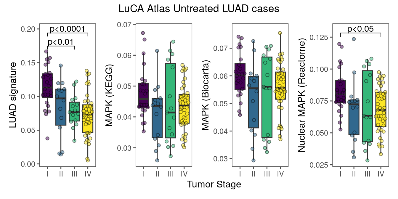
# Figure S7C -- signature scores by stage in untreated LUAD
<!-- panels: S7C -->
Per-sample treatment status and stage for the atlas, curated from the contributing studies'
own supplementary tables. `Maynard_Bivona_2020` sampled its patients longitudinally, so it
joins on `sample` to keep the timepoints apart; every other study is annotated at the
patient level and joins on `donor_id`.
```{r}
tx_f <- here("paper_data", "luca_treatment_annotation.csv")
if (!file.exists(tx_f)) {
  cli::cli_abort(c("{.path {tx_f}} not found.",
                   "i" = "Figure S7C needs the curated per-study LuCA treatment annotation."))
}

luca_treatment <- read.csv(tx_f)
stopifnot(!any(duplicated(luca_treatment$obs_join_key)))

df_tx <- df %>%
  mutate(obs_join_key = ifelse(study == "Maynard_Bivona_2020",
                               as.character(sample), as.character(donor_id))) %>%
  left_join(
    dplyr::select(luca_treatment,
                  obs_join_key,
                  tx_treatment_status = treatment_status,
                  tx_resolved_stage = resolved_stage),
    by = "obs_join_key"
  ) %>%
  mutate(
    # Every LUAD cancer-cell sample is annotated, so this only guards the panel: an
    # unannotated sample is not naive, and a named state keeps it out where an NA would not.
    tx_treatment_status = replace_na(tx_treatment_status, "not_annotated"),
    tx_resolved_stage = ifelse(tx_resolved_stage %in% c("IIIa", "IIIb", "IIIc"), "III", tx_resolved_stage)
  )

naive_df <- df_tx %>%
  filter(tx_treatment_status == "naive")

# Published panel: 93 treatment-naive LUAD samples from 81 patients.
stopifnot(nrow(naive_df) == 93)
```
```{r, fig.width = 7, fig.height = 3.5}
mapk_sigs <- c(
  "LUAD_GIRARD" = "LUAD signature",
  "KEGG_MAPK_SIGNALING_PATHWAY" = "MAPK (KEGG)",
  "BIOCARTA_MAPK_PATHWAY" = "MAPK (Biocarta)",
  "REACTOME_MAPK_TARGETS_NUCLEAR_EVENTS_MEDIATED_BY_MAP_KINASES" = "Nuclear MAPK (Reactome)"
)

mapk_pls <- map(names(mapk_sigs), .f = function(sig) {
  naive_df %>%
    ggplot(aes(x = tx_resolved_stage, y = .data[[sig]], fill = tx_resolved_stage)) +
    geom_boxplot(outliers = F) +
    geom_quasirandom(pch = 21, show.legend = F, alpha = 0.5) +
    scale_fill_viridis_d() +
    theme_few() +
    ggpubr::geom_pwc(label = "p.adj.signif", symnum.args = symnum_0.1, hide.ns = T) +
    labs(x = "Tumor Stage", y = mapk_sigs[[sig]], fill = "Tumor Stage")
})

pcomb <- wrap_plots(mapk_pls, nrow = 1, guides = "collect", axes = "collect_x") +
  plot_annotation(title = glue("LuCA Atlas Untreated LUAD cases"),
                  theme = theme(plot.title = element_text(hjust = 0.5))) &
  # Headroom for the significance brackets, which sit above the highest point.
  scale_y_continuous(expand = expansion(mult = c(0.05, 0.075))) &
  NoLegend()
ggsave(pcomb, file = here("plots", "luca_atlas_mapk_sigs_by_stage_untreated.pdf"), width = 7, height = 3.5)
pcomb
```